the page with geotechnical engineering resources and educational materials
Author: Don Warrington
Hawthorne, N.J. (January 30, 2020): Deep Foundations Institute (DFI) Educational Trust and the Terracon Foundation announce the establishment of the DFI Educational Trust/Terracon Consultants Scholarship Fund, which will provide scholarships to engineering students attending any […] The post DFI Educational Trust and Terracon Announce a New Scholarship Fund appeared first on GeoPrac.net.
Note: since this was originally posted, it has been extensively revised. There are better ways of presenting this information than are given in most American geotechnical textbooks and hopefully you will agree.
Students and practitioners alike of geotechnical engineering have learned and used Boussinesq elastic solutions for stresses and deflections induced in a semi-infinite space by structures at the surface. Although these solutions are very idealized and have many limitations, they’re still useful.
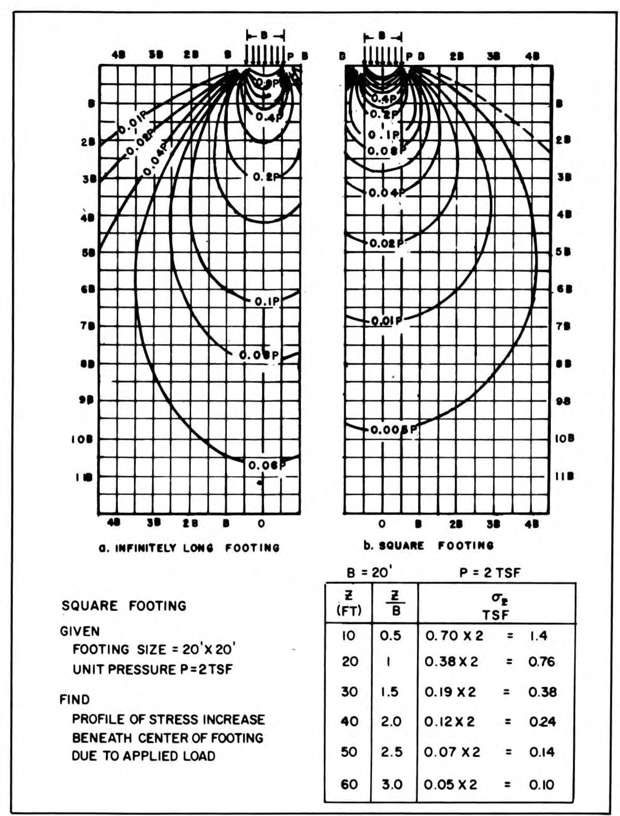
For the most part engineers have implemented these solutions–especially for loads other than point or line loads–using charts. This chart, from Naval Facilities Engineering Command (1986)–DM 7.01, Soil Mechanics, shows the isobars for stresses induced by strip and square foundations.
In addition to being hard to read (a fault which has been fixed in many of the books that have cribbed this chart) it requires a great deal of interpolation to use it and many others. In the past, the computational demands of using analytical solutions put them out of reach for practical use and educational purposes. That’s no longer the case; however, some of those solutions are difficult to find. This piece attempts to bridge that cap and set forth analytical solutions that can be used, along with a spreadsheet to implement at least some of them.
Assumptions of the Solutions Presented
They assume that the load is applied to a linear elastic, homogeneous semi-infinite space.
They assume that the foundation is completely flexible; rigid (or intermediate foundations) are not considered.
They do not consider strain-softening hyperbolic effects. These are extensively discussed in this monograph. It is more than likely that, for the cases presented here, a homogenized value for the modulus of elasticity can be arrived at, perhaps by using the methods used in the linked monograph for the toe.
Principally the vertical stresses will be considered.
All of the loads on the foundation are uniform.
Stresses Under Strip Loads
The simplest case for this set of foundation geometries is the strip load, which reduces a three-dimensional problem to a two-dimensional one. The problem is illustrated (and a point under consideration located) in the figure below, modified from Tsytovich (1976).
Diagram and Variables for Strip Load Problem, from Tsytovich (1976)
where is the uniform pressure on the foundation in load per unit area, and is the width of the foundation, usually expressed in American practice as . The angles are as shown. The stresses are as follows:
If we rewrite these equations thus
we thus have defined three influence coefficients (the “K” variables) which we can use to generalise the results.
Given the foundation width or and the angle , any point in the half space can be defined. They can be related to the Cartesian coordinates as follows:
At the base of the foundation, and , which means that the soil stress is equal to the foundation pressure , as we would expect. The stress is zero at the surface away from the foundation.
The tricky part of this is in determining from the geometry of the system and the desired location of the point in question. For students, probably the simplest way of doing this is to use CAD software. Alternatively we could also directly compute the stress from the z and y coordinates directly; for the vertical stresses only,
For stresses under the foundation centre, this influence coefficient can be reduced to
All three influence coefficients can be computed and tabulated in general. Using the two coordinate ratios and , the tabulation of these coefficients is shown below.
Influence Coefficients for Determination of Component Stresses for the Strip Load Problem (from Tsytovich (1976))
A couple of interesting graphics can be shown from these relationships.
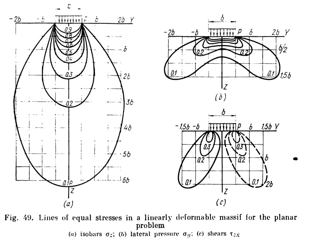
The first is the graphical representation of the tabular data of the table above, shown below.
Graphical Representation of Stresses under a Strip Load, from Tsytovich (1976)
It is interesting to note that, at the centre axis under the load, the z-direction stresses are at their maximum as a function of depth. The shear stresses along that axis are zero, and are at their maximum under the edges.
Another interesting graphical representation are the stress ellipses, whose major and minor axes denote the principal stresses. These always are along the line of the angle , not necessarily to the centre of the foundation.
Stress ellipses under a strip load, from Tsytovich (1976)
The elastic stress computations can be used to estimate the lower bound permissible stresses for bearing capacity failure, as is shown here. The direction of the principal stresses is an important part of that derivation.
Stresses under Square and Rectangular Loads
These are well known, and most engineers and engineering students have used the “Fadum charts” as shown below to obtain the solution.
Both the strength and the weakness of the charts is that the stresses computed are under the corner of the rectangle/square. It is a very specific position, but by using superposition (permissible with elastic, path-independent solutions) we can add and subtract rectangles to obtain the stress at just about any point under or near the structure in question.
Another weakness of the Fadum chart, however, is that it’s hard to read. Fadum made the results dimensionless in such a way that m and n are interchangeable, which is certainly justified by the theory, but dispensing with that can make for a solution that is easier to read. Now, of course, the increase in computational power makes use of the equations that generated the Fadum chart more accessible, but for everyday work a solution that allows for either is the best.
Bowles (1996) presented the solution that has been most widely disseminated, but ultimately most solutions are based on that of Newmark (1935). His solution was as follows:
where B, L and Z are the width, length and depth of the point of interest below the corner.
Let us, following Tsytovich (1976), define three different dimensionless variables thus:
(the influence coefficient for the vertical stresses)
(the aspect ratio of the foundation or the part of the foundation of its length (longer side) divided by its width (shorter side)
the aspect ratio of the foundation or part of the foundation of the depth from the corner to its shorter side.
As was the case with Bowles (1996), which equation you actually use depends upon what quadrant the second (arcsin or arctan) term ends up in. The equations using these dimensionless variables are as follows:
If :
If :
The “border” between the two equations is shown below.
Plot of Curve where the form of the equations change.
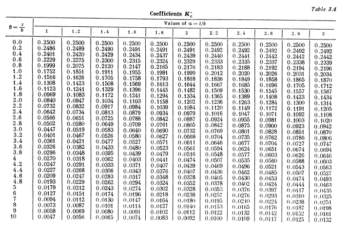
A table representing the results is below.
The biggest drawback to this is that the sides aren’t as interchangeable as with the Fadum charts, but since for rectangles L>B customarily that shouldn’t pose much of a problem.
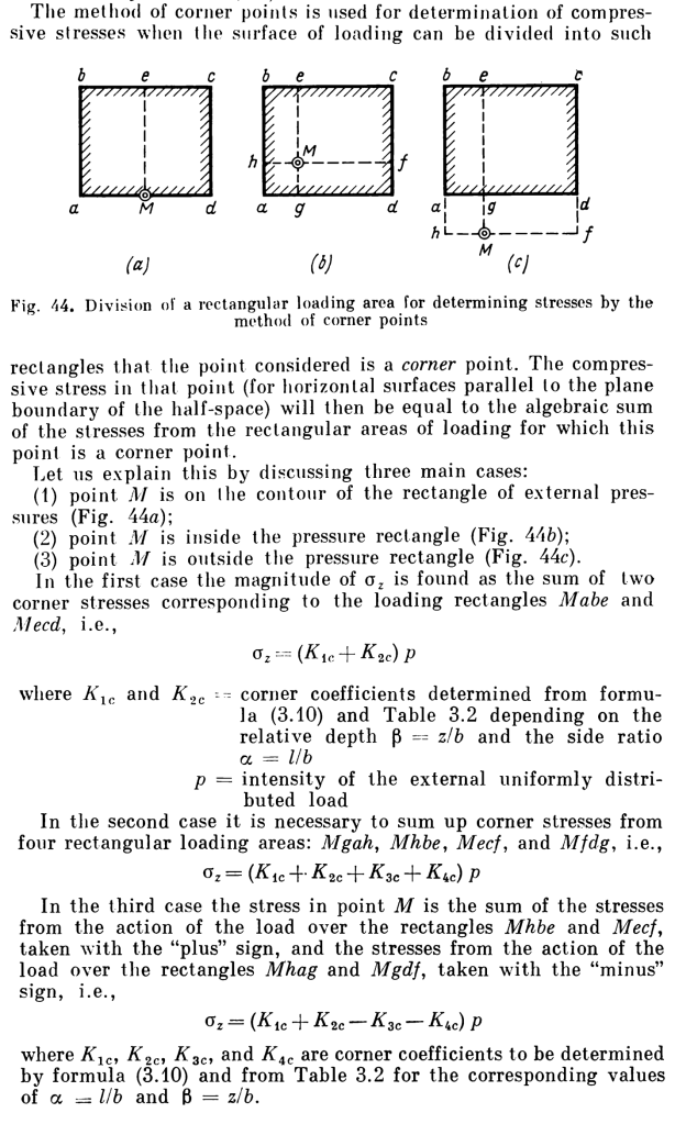
Obviously we might be interested in points below the surface other than those directly under the corner. This can be done using superposition (which is available since all of this is elastic theory and thus the results are path independent.) Below is a description of how it is done, using charts with a plan view of the foundations:
Method of using superposition to determine the vertical stress at a point under a foundation at a point other than a corner. Note that all of the K factors can be determined using Table 3.4 above. From Tsytovich (1976)
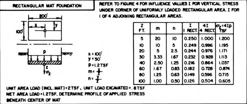
As an example of Case (b), consider determining the stress in the centre of the foundation, as is the case in this example, from NAVFAC DM 7.01:
This problem was solved using the Fadum Chart. To use the method shown, we simply need to realign our variables. For the stresses at the centre, the foundation being analysed is one fourth of the original. So we set L = 100′ and B = 50′, which means that . The values for are shown as follows:
Z
5
0.1
10
0.2
20
0.4
30
0.6
40
0.8
60
1.2
80
1.6
100
2
The influence coefficients can be determined either by the equations or the table. They should be identical to those shown in the example; however, since those were probably taken off the chart, there will be small variations. Once they are determined, they should be multiplied by 4 for the complete solution.
It is interesting that the problem reduces the net pressure on the foundation by the effective stress at the base of the foundation. This is one way to deal with this problem; it is used in Schmertmann’s Method for settlement. You need to look at how you plan to use the results before doing this. It is important to note, however, that no matter how you handle this the value of Z is the distance from the base of the foundation, not the surface of the soil.
Diagram for problem where there are two different pressures and two different foundations, from Verruijt (2007)
It should be noted that adding the influence coefficients K assumes that the p is the same for the whole foundation. The method can be expanded to foundations where that is not the case and an example of this is given in the Rectangular Elastic Solutions Spreadsheet, featuring a problem taken from Verruijt, A., and van Bars, S. (2007). Soil Mechanics. VSSD, Delft, the Netherlands., who solve the problem using Newmark’s Method. The difference is that, while the description from Tsytovich adds K factors, the problem here adds and subtracts stresses. Using the formulae the superposition method is more precise than Newmark’s Method.
Another description of the superposition method, from NAVFAC DM 7.01 (1986)
Deflections of Squares and Rectangles
Elastic solutions can be used to predict both stresses and deflections. Most engineers are familiar with tables such as this, and these are still used for initial deflections and deflections in media such as intermediate geomaterials (IGMs.)
Keeping in mind that we are still assuming the foundation to be perfectly flexible relative to the soil/IGM/rock, the equation for the deformation of the foundation is as follows:
where
settlement of the foundation at the point of interest
influence factor, given in the table below
uniform pressure on the foundation
smaller dimension of rectangle or dimension of square side
Poisson’s Ratio of the soil
Modulus of elasticity of the soil
The factors are given below, both for a soil layer of large depth and one of limited depth .
Table for Values of Influence Coefficients, from Tsytovich (1976)
The table also includes values for rigid foundations, which we will not consider here.
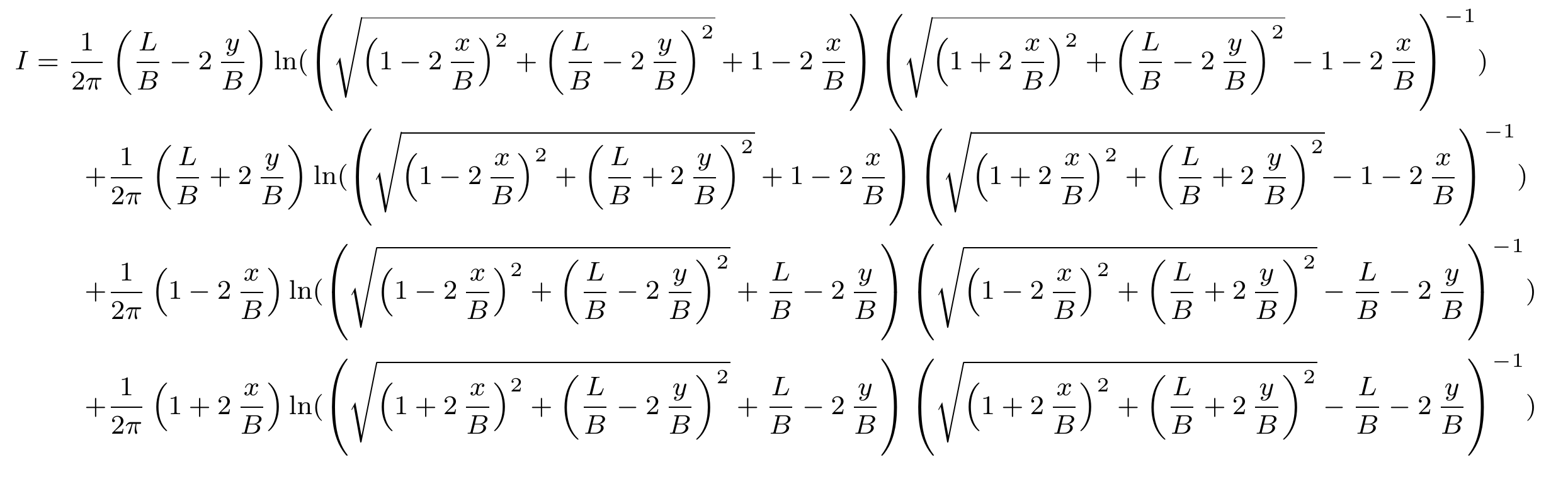
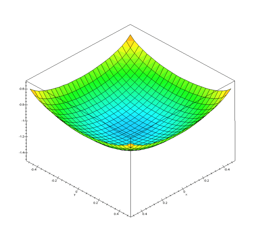
As was the case with the stresses under square or rectangular foundations, the equations for the deflections are quite involved. For these foundations, assumed flexible and uniformly loaded, the influence coefficient is computed by the following equation (Perloff and Baron, 1976):
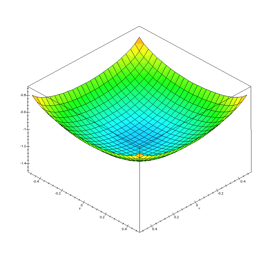
In this equation the origin is assumed at the centre of the foundation, not at the corner. Thus, the values of x and y are as follows: -B/2 < x < B/2 and -L/2 < y < L/2. As an example of how this looks over an entire foundation, consider the case of B=L=1 (a square foundation.) The influence coefficient of the foundation can be plotted as follows:
It is easy to see what is meant by “flexible” foundation.
The problem with this formula is that, if blindly followed mathematically (just inserting the variables) singularities quickly arise both along the edges or at the corners. Symbolically solving (and taking a few limits) get around this. For the mid-point of the edges,
And at the corners,
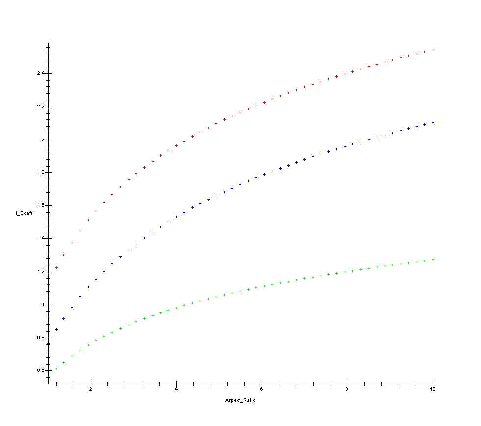
A plot of the same functions mentioned in the table above from the formulae is below.
Rectangular foundation deflection for the center (red,) mid-point of the long side (blue,) and corner (green) for various aspect ratios of L/B
The center deflection can be found by either substituting x=0, y=0 into the first equation or by using the equation
Some Observations
Use of theory of elasticity in this way has been employed in foundation design for a long time, even with the inherent limitations of the method. It gives reasonable approximations for either initial deflections or for deflections of IGM’s. For implementation on a recurring basis, use of the formulas allows a more precise implementation of these methods but not necessarily a more accurate one, but the errors inherent in reading charts are eliminated.
In our opinion it is possible to improve the accuracy of the method by improving our understanding of the elastic modulus of the soil, and in particular strain-softening near the foundation itself.
The deflections are probably the less satisfactory products of this theory than the stresses. No foundation is either purely flexible or rigid, and using a purely flexible foundation produces larger variations in deflections than one would expect in reality. Also, the typical rule of thumb that foundations with an aspect ratio larger than 10 can be treated as continuous/infinite foundations is reasonable for stresses but not for deflections, and in fact the chart shown above was truncated. Whether this is reflected in reality is another question, and this too doubtless relates to the flexibility of the foundation.
Other References
Bowles, J.E. (1996) Foundation Analysis and Design. Fifth Edition. New York: McGraw-Hill.
Perloff, W.H., and Baron, W. (1976) Soil Mechanics: Principles and Applications. New York: Ronald Press.
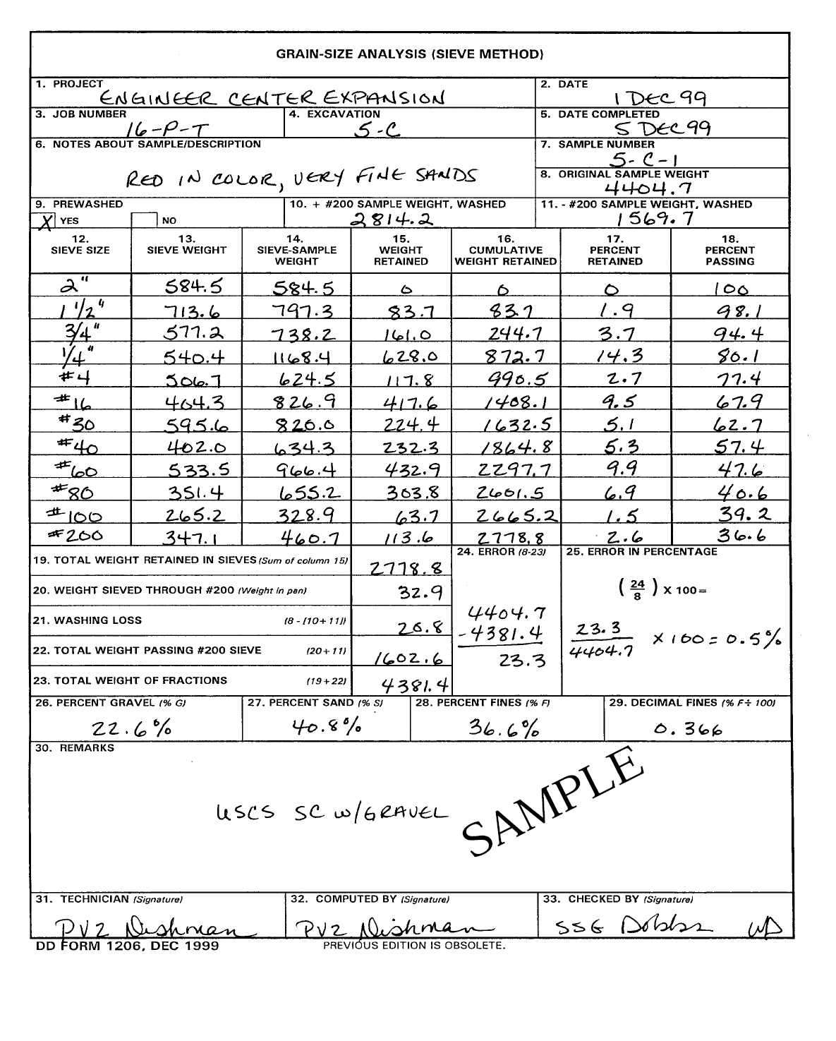
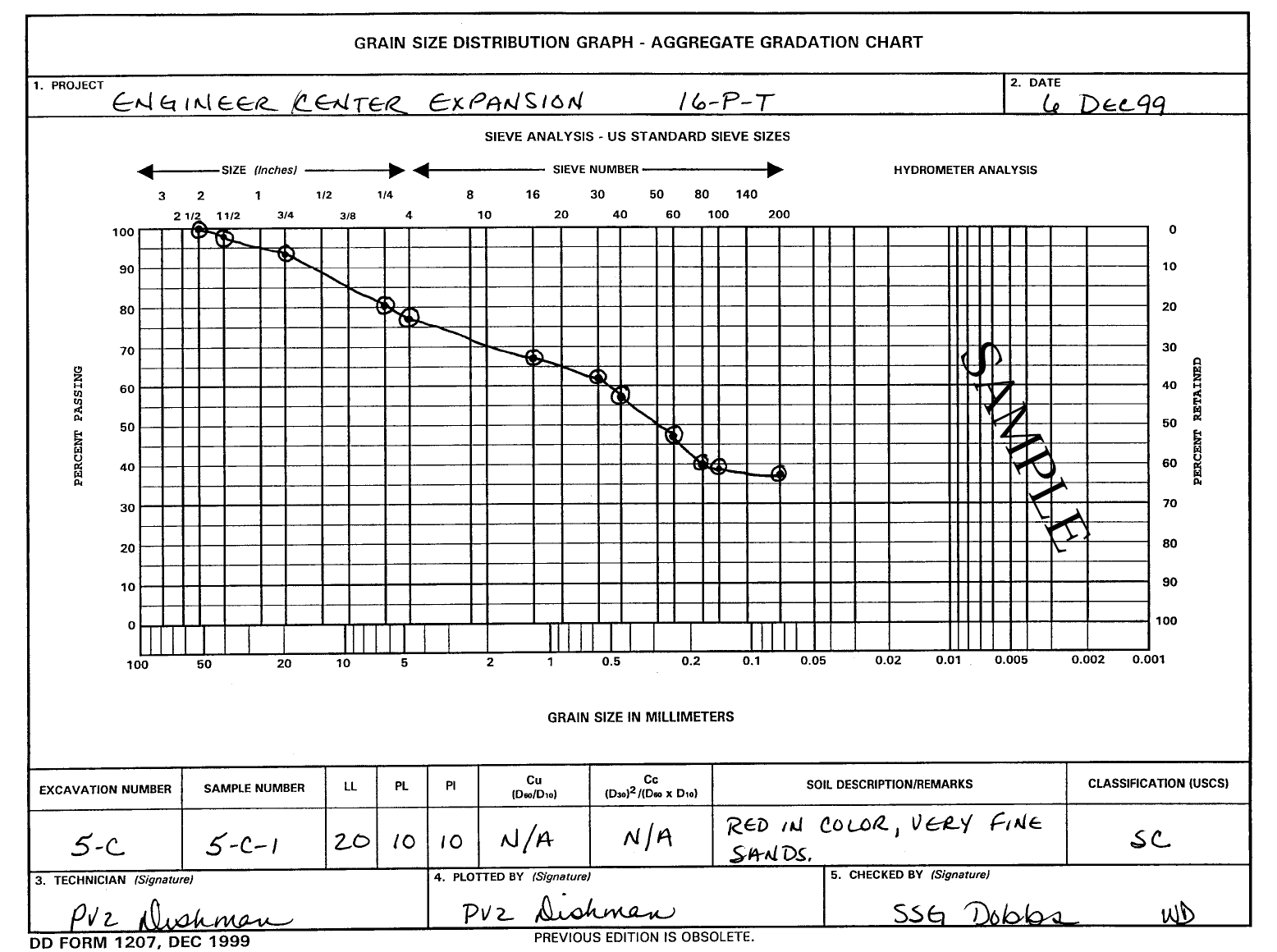
This is a sample sieve analysis result. For the lab (especially when sample washing is involved) it can get this complex, and the procedure is described in Materials Testing. To look at this more schematically (and this is common for most “textbook” problems) the following simplifications are done:
There are no losses in the process of sieve analysis. This is obviously unrealistic but these should be kept to a minimum. For textbook type problems this means that Blocks 8 and 23 are the same.
The tare (sieve or pan) weight is removed from consideration. This means that typically Column 15 is the first column in the problem, given the soil weights retained on each sieve. The weight that “hits the pan” is in Block 22.
Washing losses and errors are not considered, which means that Blocks 21 and 24 are set to zero.
With these out of the way, we can proceed to the analysis. The top sieve in the stack (the 2″ sieve) retained no soil (it doesn’t always happen this way) so it has zero soil retained and all passing. The next sieve (the 1 1/2″ sieve) retained 83.7 g (Column 15.) For the cumulative weight retained (Column 16) we add the value of Column 15 just above it to this one, thus 0 + 83.7 = 83.7 g. The next sieve (the 3/4″ sieve) retained 161 g, so for the cumulative weight retained for this sieve we add in the same way, thus 83.7 + 161 = 244.7 g. We keep going in the same way “down the stack” until we have all of the cumulative weights retained for each sieve computed.
This is terrific, but what we really need is the percentages of the total sample each cumulative retained value represents. This is what goes in Column 17. These values are obtained by dividing each result in Column 16 by the total sample weight in Block 23 and multiplying them by 100 to obtain a percentage. In this way, the cumulative percent retained for the 2″ sieve is obviously zero, for the 1 1/2″ sieve 83.7/4381.4 x 100 = 1.9%, for the 3/4″ sieve 244.7/4381.4 x 100 = 3.7%, and so on.
We can also compute the percent passing. An easy way to do this is to start by noting that 100% passes the whole sieve stack. We can than successively subtract the cumulative retained percentage as we go down. Thus the percentage of the 2″ sieve is again obviously 100 – 0 = 100%, for the 1 1/2″ sieve 100-1.9 = 98.1%, for the 3/4″ sieve 98.1-3.7 = 94.4% (note that we use the percentage passing from the previous sieve each time) and so on.
We then plot the results on the sieve curve as follows:
It’s a temptation these days to use a spreadsheet and its semi-logarithmic plotting features. I would avoid this: using a dedicated form like this has two advantages:
It lines up the grain sizes and sieve designations for you.
It can be plotted either from the percent passing size (left) or percent retained side (right.)
It’s also possible to use a tool such as the Spears Lab Spreadsheet, but this takes a lot of practice and is a little tricky to use, especially for “textbook” type problems where the tare is not considered. It’s easy to get a really stupid looking result; I have seen quite a few over the years.
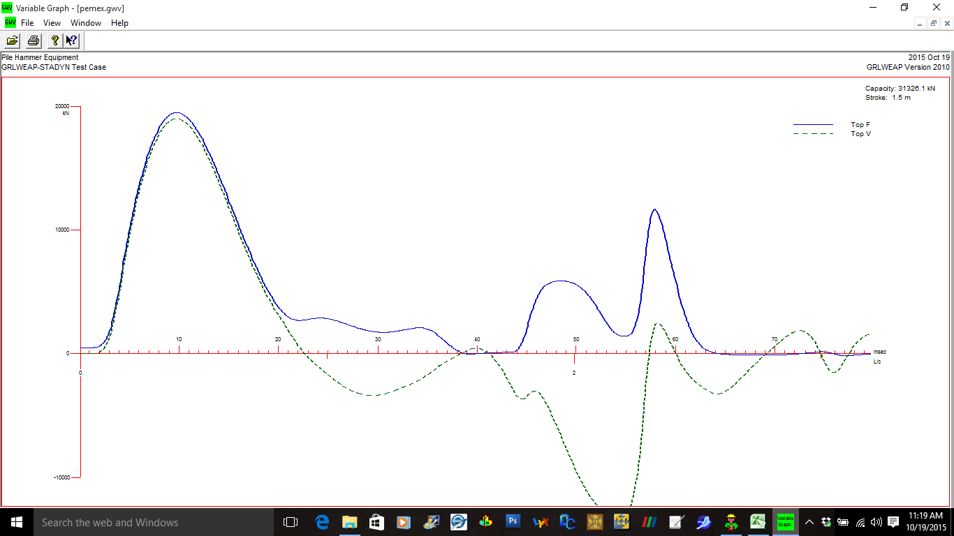
While looking through some files, I found these from the original STADYN project, from the comparison case with GRLWEAP. I’m passing these along to give you an idea of the graphical output of this program. My thanks to Jonathan Tremmier of Pile Hammer Equipment for allowing me to use this copy of GRLWEAP.
This is the “main screen” of GRLWEAP, giving a schematic view of the hammer/pile/soil system and allowing for input of parameters.
This is the “bearing graph” output of the program, also giving a graphical representation of the system.
This is the force-time and impedance*velocity-time trace for the pile head. Comparing the two is an important element when this data is gathered in the field.
This ceremony took place last month at UTC. I was the “matchmaker” for the agreement; after UTC signed a similar agreement with Covenant College, I thought “why not Lee?” Being well embedded and known in the Church of God (and my wife a Lee graduate,) I reached out to Dr. Debbie Murray, Lee’s Vice President for Academic Affairs. Her response and that of from Dr. Paul Conn, Lee’s President, was positive. Then I approached UTC’s Dean of the College of Engineering and Computer Science, Dr. Daniel Pack, and he was receptive. The rest, as they say, is history.
An articulation agreement like this specifies that the students spends three years at Lee and two at UTC, obtaining an engineering degree at the end. Making this available is a step forward for both institutions. Additionally Lee students won’t have to make a major move (if any) to complete their degree, since the two institutions are about 30 miles apart.
This has been one of the most gratifying things I have been involved with both in my years in the Church of God and at UTC.


 is the uniform pressure on the foundation in load per unit area, and
  is the width of the foundation, usually expressed in American practice as
  . The angles are as shown. The stresses are as follows:


 , any point in the half space can be defined. They can be related to the Cartesian coordinates as follows:

 and
and  , which means that the soil stress is equal to the foundation pressure
![K_z=\frac{2}{\pi}\left[arctan\left(\frac{b}{2z}\right)+\frac{bz}{\frac{b^2}{2}+2z^{2}}\right],\,y=0](https://s0.wp.com/latex.php?latex=K_z%3D%5Cfrac%7B2%7D%7B%5Cpi%7D%5Cleft%5Barctan%5Cleft%28%5Cfrac%7Bb%7D%7B2z%7D%5Cright%29%2B%5Cfrac%7Bbz%7D%7B%5Cfrac%7Bb%5E2%7D%7B2%7D%2B2z%5E%7B2%7D%7D%5Cright%5D%2C%5C%2Cy%3D0+&bg=ffffff&fg=777777&s=0&c=20201002)
 and
and  , the tabulation of these coefficients is shown below.
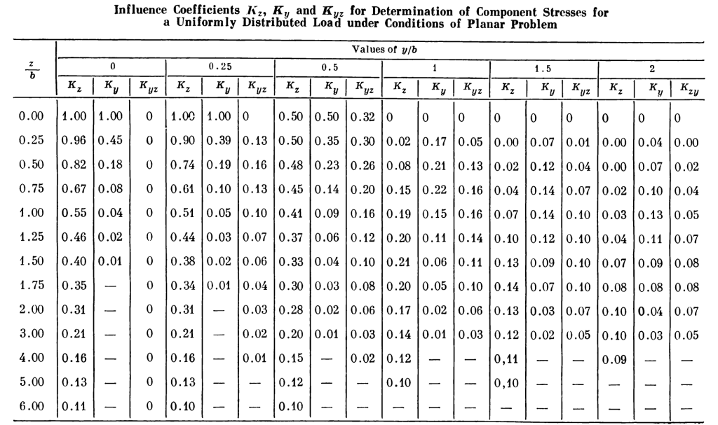
 , not necessarily to the centre of the foundation.
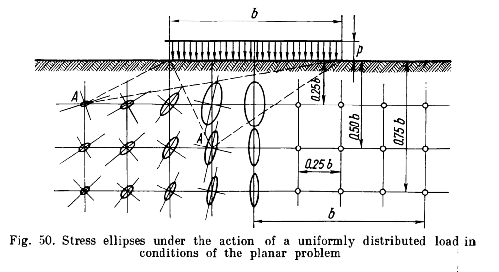


 (the influence coefficient for the vertical stresses)
 (the aspect ratio of the foundation or the part of the foundation of its length (longer side) divided by its width (shorter side)
 the aspect ratio of the foundation or part of the foundation of the depth from the corner to its shorter side.
 :
:
 :
:


 . The values for
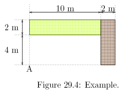


 settlement of the foundation at the point of interest
 influence factor, given in the table below
 uniform pressure on the foundation
 smaller dimension of rectangle or dimension of square side
 Poisson’s Ratio of the soil
 Modulus of elasticity of the soil
 are given below, both for a soil layer of large depth and one of limited depth
  .
.