Category: Academic Issues

This post has been a long time coming. I’ve been teaching engineering for a quarter century now, and when not doing that developing sites like this so that engineers (and others) can learn more about design and construction of geotechnical structures (and all structures, to varying degrees, are geotechnical unless they float on the water, in the air or in space.)

I come from a long time of technically educated people, as visiting my sites vulcanhammer.info and Chet Aero Marine will show. My great-grandfather learned the basics from Smith’s Mechanic at the University of Illinois in the 1870’s and both he and his brother had successful careers as naval architects. So I come to this debate with a long family history in this profession and many years of experience in the design and application of construction equipment, which is why my teaching straddles both Civil and Mechanical engineering. Many of those who have visited this site are familiar with my Soil Mechanics, Soil Mechanics Laboratory and Foundations courses. After teaching these for a long time, it was evident that our students weren’t “getting it” on what I thought were fundamental concepts. Moving to Lee University and teaching Statics and Dynamics only confirmed those suspicions. Added to my experience with Fluid Mechanics Laboratory and later Fluid Mechanics and this post is the sum of my reflections on this experience.

For those of you who would like a more specifically geotechnical focus, you might find my 2024 piece My Response to Rodrigo Salgado’s “Forks in the road: decisions that have shaped and will shape the teaching and practice of geotechnical engineering” and an announcement interesting.

First, let’s look at the challenges we face:

The Challenges

1. The growth in the use of numerical methods while the curriculum still emphasizes the use of “hand calculations.” A lot of that is driven by testing; as my CFD professor said after a disastrous midterm (and it was a 500 level course!) testing isn’t perfect but it’s the best thing we have to evaluate whether students are learning the material. The problem with this is that engineers tend to regard results that a computer produces come from Mt. Sinai (the “black box” phenomenon”) and this does not lead to good engineering practice.
2. We all too frequently lose sight of the fact that our first purpose is to teach people how to think, not just how to make computations or apply formulae. The latter is especially tempting in geotechnical engineering because so many of our formulae are empirical to varying degrees, but we’re not the only people with this problem.
3. AI, for all of its potential and actual benefits, encourages mental laziness. There, I said it. That’s the root problem with AI, and everything else only leads to that. We don’t need mental laziness in this profession or any other for that matter.
4. Students’ ability to visualise problems has deteriorated with the growth in computer graphics, from CAD to all kinds of 3D modeling. One thing that vanished before I got into this was students’ ability to draw, but we need to make CAD a solution rather than a problem.
5. Engineering curricula suffer from being squeezed into a smaller and smaller portion of the course of study engineers are required to take. State school people will recognize the fight with “GenEd” people but it’s not only a problem with state schools.

This last point is not only fueled by the amour-propre of non-STEM faculty; it comes from something that I’ve noticed over the years on Positive Infinity: there is a deep-seated fear that engineers and other scientifically trained people, without the benefit of a liberal arts education, will take over society and enforce a cold, uncultured ethic on everyone else. But that exposes one of the main weaknesses of the American educational system: we warehouse people for over a decade before expecting colleges and universities to impart to them “culture” and “critical thinking skills.” Both of these should be formed long before they step into the halls of “Old Ivy” or “Old Kudzu” (the latter is becoming more important these days.) Our biggest problem is that we cannot agree on a “culture” to teach our young people let alone whether an educational institution of any kind can or should impart such things.

Having said all that, let’s get to the concrete suggestions.

Dial Back or Lose Vector Analysis in Solid Mechanics

One of the advantages of living in the internet era is that we can easily look up books from the past, especially if they’re out of copyright. Engineering education, in a sense, is moving from the oldest knowledge to the newest, the oldest coming first in the early years and as one progresses one learns the newer stuff until, hopefully, the student meets the latest when they get the “terminal degree.” (Geotech warps this process because its transition into true scientific territory is later than other disciplines.)

Now that we have archived textbooks, we can see this process in the books that are readily available. From my great-grandfather’s Smith’s Mechanic to Analytical Mechanics for Engineers to Statics and Dynamics of a Particle, both the content and the pedagogy advance. We also have the Soviet books of a newer vintage; they had a poor economic system but an excellent educational one, and produced texts such as Theoretical Mechanics and Theoretical Mechanics: A Short Course. Other disciplines show the same trend. In all cases engineers trained under these methods went on to produce excellent designs even with the lack of computational power because they were forced to develop serious engineering judgement.

Around World War II we saw in this country a shift to a more precise and analytical approach to teaching solid mechanics. A large part of that was the application of vector analysis, especially for three dimensional problems. When I was taking these courses in the early 1970’s, one could expect to use these in practice. Today that expectation was gone; all problems but the simplest are subject to some kind of numerical method. We would be better off going back to what I call “old coot statics” and dynamics (two-dimensional analysis without vectors) and leave the three-dimensional problems to the numerical methods. Students today, especially with their visualisation problems, need to concentrate on developing their thinking skills and not get bogged down in vector analysis, which in turn is similar enough to linear algebra to develop confusion of both.

An example of the contrast between old coot statics and vector statics can be seen in the example Vector Statics and “Old Coot” Statics: An Example. In the example the two computational methods are set out side by side; the vector analysis is considerably more complicated.

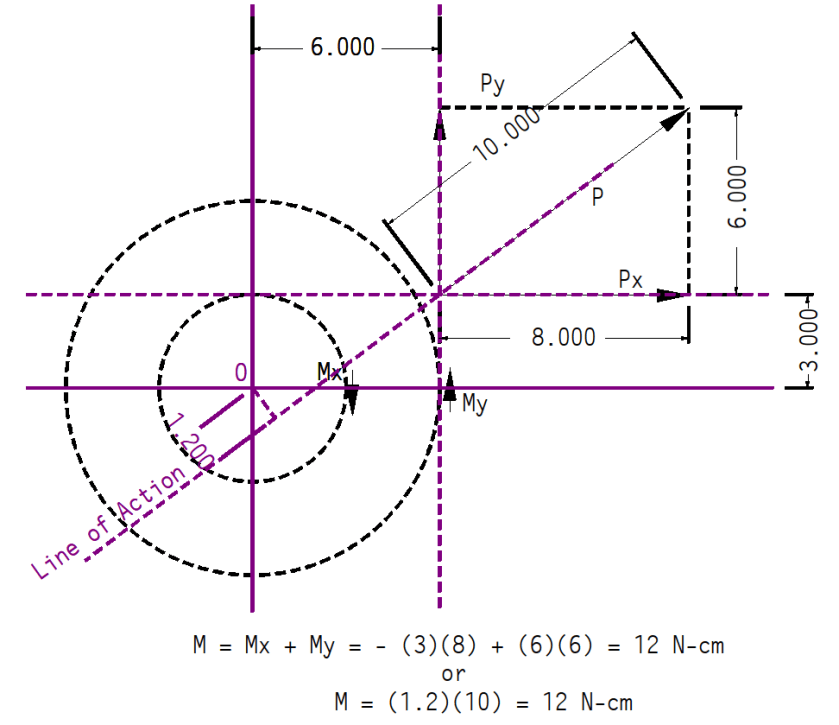
Vector analysis also obscures the fact that a moment is the product of the force and the perpendicular moment arm from the point of application to the line of action of the force. This is illustrated in An Example of 2D Moment Computation. In fact that’s the key problem to vector analysis: the student gets bogged down in setting up the problem rather than understanding its nature.

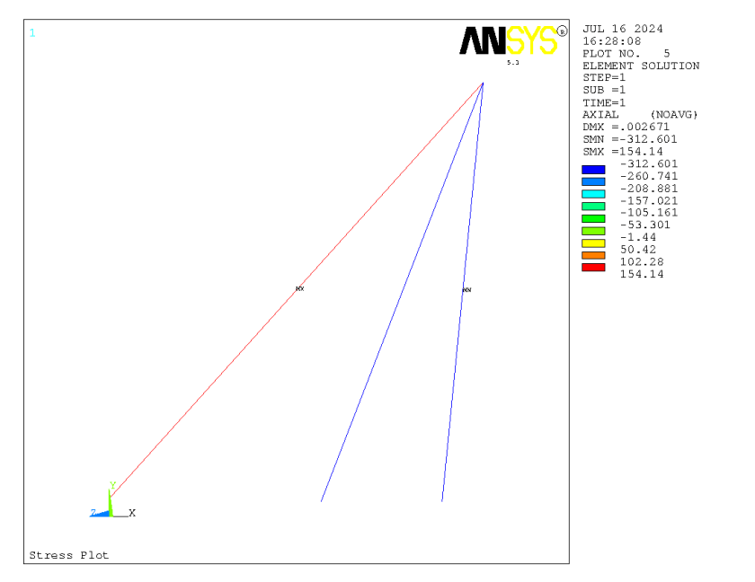
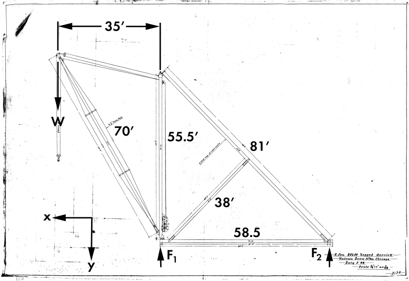
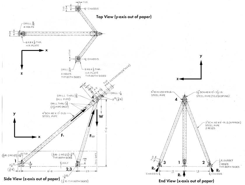
Problems–especially three-dimensional ones–are best left to numerical methods and emphasis on two-dimensional problems for basic understanding would be a better approach. The last example I’d like to give is An Example of 3D Vector Statics With a Simple Truss. Here we have a problem where (as you can see in the example itself) the vector solution is just too much for the problem; we could either a) use a numerical method or b) split the problem into two two-dimensional problems, one in the x-y plane and the other in the 2-3-4 plane.

The solution in ANSYS (I know this is an old version, we run on a low budget on this site) is below.

I’m aware that vector analysis is well embedded in the teaching of mechanics, but I think it’s time to take a serious look at the problem.

Bring Back Graphical Methods

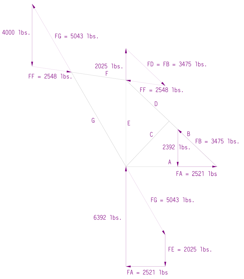
One hallmark of engineering practice in the past was the use of graphical methods to resolve forces and perform other tasks which would be computationally expensive. The advent of the calculator and later the computer into the profession gave the impression that graphical methods were a thing of the past.

With CAD that’s not the case: we can solve problems with the same precision in CAD we do with either vector analysis or “old coot” statics. An example of this comes from the very first example shown; the graphical solution is given in the article Stiff Leg Derrick Part II: Truss Analysis, and can be seen below. The magnitudes were measured in CAD and the directions were done using the basic derrick layout in CAD.

Another example of a semi-graphical method that gets the short shrift these days is rotation about an instantaneous centre; I give an example of this in Solving a Dynamics Problem using the Instantaneous Centre of Rotation with a Vulcan Design.

Graphical methods will assist visualisation and give students a better feel for the problem, both of which they need in their development as engineers.

Distributed Loads and Concentrated Resultants

This comes out of my geotech teaching but also Fluid Mechanics as well: my students struggled with the transition from distributed loads to concentrated resultants. And the distributions were the usual ones we see in geotech and Fluid Mechanics: linear, either uniform, triangular, or trapezoidal. I’m not sure what the solution is but there are two things we need to consider: a) the aforementioned vector statics and b) the inclusion of algebraically complex loadings with polynomial or other higher order equations. As a practical matter it’s unlikely that a complex loading encountered in practice will obey these equations but will more likely require a stepped type of loading of some kind, which in turn begs a numerical solution.

Keep Basic Fluid Mechanics Basic

Fluid Mechanics has experienced much of the same transition as solid mechanics. From books like Hydraulics and Fluid Mechanics to those we usually teach from now, an emphasis on practical fluid mechanics has been lost. In my own career I have found that many of the problems I had would have been much easier to see if the curriculum I was taught under had stuck with a more basic approach (and books which emphasise that do exist, as you can see from my own course.) What we need is to do the following: a) save much of the more theoretical treatment for an advanced course, paralleling that of mechanics of materials, and b) integrating that type of material into basic Computational Fluid Dynamics, which is a necessity for many fluid mechanics problems.

One other thing worth mentioning is that, in the past, solid and fluid mechanics were more integrated, as you can see in books from Smith’s Mechanic to Mechanics by S.P. Strelkov. We might consider some of this if we decide to seriously rearrange how we teach these subjects.

Putting a Wrap

This is not meant to be an all-inclusive list, and I realise that some of these suggestions will be controversial. Today it’s fashionable in higher education, as it has been down the line for many years, to emphasise the pedagogy methods as opposed to the content. But a simpler, more straightforward approach to subject would lend itself to easier pedagogy; the two aren’t unrelated. The tendency to push practitioners out out teaching–one driven in part by our accreditation process–has left many with an unclear understanding of what is required of engineers once they graduate. There are many issues we face; this piece is only meant to start the conversation, not finish it.