A recent inquiry revealed that the literature on this site and vulcanhammer.info has a difference of design procedure for anchored sheet pile walls.
In order for a deadman anchor to be effective, it must be beyond the failure envelope. Here we present two ways to insure that this is so.
The first is shown above: it is taken from NAVFAC DM 7.2, although it has been in many publications over the years, including NAVFAC DM 7.02 and Sheet Pile Design by Pile Buck. It shows the point at which the failure envelope starts as the “estimated point of zero moment in wall.” That can be determined using software such as SPW 911.
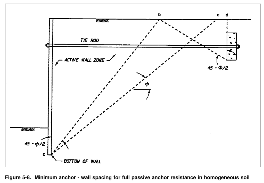
The second is shown below, from EM 1110-2-2504, and shows the same point at the bottom of the wall.
If you have any comments about either of these methods, or which one you prefer and why, let us know in the comments.
The current predominant regime in pile dynamics has been around for over half a century now. With tweaks and improvements in computer power and hardware, it has enabled us (well, most of us) to jettison the problematic dynamic formulae for capacity prediction and verification during installation. The whole system, however, relies on the 1D representation of pile/soil interaction to be accurate and the optimization algorithm to find the solution to the inverse problem. Both of these are subject to the kinds of improvements we see in other fields.
Getting to this point was not an easy or straightforward task, both because of the application itself and the code/regulatory environment in which we operate. Much of the struggle to get the current methodology accepted was an uphill battle against the existing “we’ve always done it this way” mentality which settles in, and no doubt this will be the case with a new generation of pile dynamics methodology. But there are some difficult challenges inherent in the physics of this problem, most of which stem from the nature of soils themselves.
I ran into many of these challenges during my study which led to Improved Methods for Forward and Inverse Solution of the Wave Equation for Piles. One colleague from an institution in a neighbouring state felt that my effort was “too ambitious.” He’s probably right, which is why he’s in administration now. But my objective was for this study–and the subsequent papers to fine tune the method–to be a convesation starter, and this paper’s citation of my work is evidence that this is taking place. I sense that efforts to “move the football down the field” in this discipline are taking place, and am gratified to be a part of that effort.
Comments on the Paper Itself
Strictly speaking this paper only has the inverse method as a commonality with my own study. In this case the researchers are dealing with a drilled shaft and are trying to back analyse static capacity. While this sidesteps the rate-dependent problem between dynamic signals and static response, it brings other factors into play, some of which are definite weaknesses in the paper and others where the jury is still out.
Optimisation Technique
Let’s start with one which falls into the latter category: the optimisation technique they chose, which was the Davidon-Fletcher-Powell method. The purpose of optimisation techniques is to find the minima and maxima of “equations” (often they can be expressed in this way, but in this business frequently they can’t) and thus the best solution to the problem. The classic example of this (and one frequently used to test optimisation techniques) is the Rosenbrock Equation, which is
and is plotted as shown below for a =1 and b = 100.
This has challenged optimisation techniques for a long time. The problem with using something aimed at problems like this is that, in geotechnical engineering, problems look less like this and more like relief maps. The result is having to deal with false minima. For example, if we have a canyon on top of a plateau, a false minimum would be the lowest elevation at the bottom of the canyon rather than the bottom of the cliffs of the plateau, which are generally lower. Multiple false minima are common for problems in this profession, which is one reason why we still use brute force grid optimisation in problems like slope stability. This is why I chose a polytope method for my own study, which is derivative free and “casts a wider net” on the downhill slopes of a problem. It is slow and its results not perfect but I think this is a problem that needs to be addressed if we are to use optimisation techniques for solving geotechinical problems.
My last course for my PhD degree was in Optimisation. One day our professor–Dr. Kyle Anderson, one of the most brilliant people I’ve come to know–was going on about these techniques, and as you can see Roger Fletcher’s name comes up in many of them. So I leaned over to one of my classmates and said, “Fletcher sure does play both sides of the street.” Dr. Anderson was irritated at seeing whispering, and made me repeat this to the whole class. When I did he thought for a second and said, “He does play both sides of the street.”
The Capacity Issue
In the paper at hand, the optimisation technique starts with initial values and comes to back-analysed values which are then compared to reference values. The problem here is that the reference values are based on single values of toe capacity and soil parameters, the latter of which are related to static methods of analysis. There are two problems which arise in this approach.
The first is the variability of static methods relative to the actual performance of the deep foundation. This is evidenced by the wide scatter in the results these methods return (it’s not quite as bad with drilled shafts as it is with driven piles, but it’s bad enough.)
I think this paper is an interesting study as a step towards using optimisation techniques to solve the inverse problem of pile resistance to axial load. But there are many more issues to deal with if we are to come to a workable solution for this problem.
We start with an existing technology: low-strain integrity testing of piles. A simple example of this is shown above, it’s the Pilewave program from Piletest. (Yes, I’m aware that it’s the Windows 3.1 version, if you’re interesting in running DOS and Windows 3.1 programs to save on the expense of “new” engineering software, you can visit Partying Like It’s 1987: Running WEAP87 and SPILE (and other programs) on DOSBox.)
With that distraction out of the way, note that, as the stress wave goes down and back up the pile, there is attenuation due to the interaction with the soil. In the simple demo of Pilewave, the soil resistance is constant along the shaft. But…if we could determine that the pile didn’t have defects which reflected waves, could we use information from the soil attenuation to determine the type of soil surrounding the pile at any given elevation? The answer in principle is “yes” and this paper, although not unique, it is an interesting step forward.
Pile Integrity Testing is a low-strain technique. That’s in contrast to the high-strain methods we’re used to in pile driving analysis. This one takes a leaf from the seismic refraction method (which will be featured as before in Soils in Construction, Seventh Edition) which is also a low-strain technique, as it is a geophysical method. The idea is that the pile acts as a probe into the soil; the response to exitation can be inversely analysed to determine the types of soils around the pile. As the paper notes, if you divide up the pile into enough “layers” the actual soil layering itself (based on the properties returned to you by the method) will basically emerge from the data.
As is generally the case with inverse methods, the solution is complex; it is described in the paper. There are a few comments that I would like to make as follows:
His governing equations are similar to the Telegrapher’s Equation used in Closed Form Solution of the Wave Equation for Piles and include a strain term but lack a damping term. Usually a damping term is necessary to model the energy dissapation into the soil; whether that applies to this problem remains to be seen.
Driven piles are subject to compaction and disturbance at the soil-pile interface; how this affects the results remains to be seen. The difference in soil response based on rate effects also will need to be addressed.
I hope that this research continues; I think it has potential.
As we begin a new year (for this site, it’s the 29th) we need to clarify some things that have changed regarding our book offerings.
We’ve been with Lulu publishers since 2006 (this is our twentieth year with them) and we’ve been through many changes in the publishing industry since that time. In those days we not only offered print books (our government doesn’t print their geotechnical publications any more) but also CD’s with documents. They only sold these books and CD’s on their own website.
Later they began to offer to put books “in distribution,” i.e. with places such as Amazon.com and other book sellers. We’ve been migrating our product line in that direction but have run into two problems.
The first is that distribution is expensive; these people like to take a substantial cut. This forced us to price things accordingly, although we’ve tried to keep our own cut at a reasonable level.
The second is that the requirements for a book to be in distribution changes, or more accurately the way that Lulu and these publishers enforce these requirements changes. The result is that books which have been in distribution for years are no longer there, although they’re still available from Lulu.
Our response to this is to simply keep the books in distribution which are most popular and to allow the rest still being published to stay on Lulu. The result of that is below, with our entire geotechnical book line listed. In taking books out of distribution we’ve looked at our pricing and have reduced prices on several titles.
We’d like to wish everyone who visits this site a Happy and Prosperous New Year.
A popular retired Missouri University of Science and Technology (MS&T) professor, David will be remembered for his love of teaching, his wide range of interests and knowledge, as well as his endearing sense of humor.