It’s official: Soils in Construction, the textbook I have been a co-author on for more than twenty years, is now set to have a Seventh Edition sometime in the next twelve months.
The main objective of this edition is to bring things up to date, and that especially includes the graphics. This book has been around for over fifty years and, although the photos we have used have been very good for instructional purposes, advances in graphic design make it important that these be kept up to date where this is possible.
If you or the organisation you work for have photos or diagrams of geotechnical construction work that you think might be useful for the book, go to the contact page and send a message. Full credit (but no monetary compensation) will be given for submissions that are actually used.
I recently received in inquiry from an organisation which has proposed a shallow foundation of an embankment. They used (wisely IMHO) an FEA analysis to estimate the settlement. The owner’s response was that, since their result was a little greater than Hough’s Method, and Hough’s method reputedly overestimates the settlements by a factor of 2, that the FEA analysis overestimated the settlements. They referred this person to my posts Getting to the Legacy of B.K. Hough and his Settlement Method and Closing the Loop (or at least trying to) on Hough’s Settlement Method, which is evidently about the only ongoing discussion of the topic around these days.
Both of these posts have two objectives: a) they attempt to trace the development of the method, both by Hough and those who came after, and b) to begin the journey to a resolution of the accuracy of the method. The problem with both of these is that the problem is simple to state but, because of the nature of the evidence, difficult to resolve. I’ll start with a brief review of these two objectives and then set forth a worked example (something that is admittedly lacking in my first two posts) to see how things work out. I’ll end with some thoughts on how to more accurately determine the values of C’, which is the core issue with this method.
The Method and Its Development: A Review
“The SPT is a dynamic test, while soil bearing capacity is a matter of statics, interpreting one in terms of the other is analogous to determining the bearing capacity of piles from pile driving formulas. Consequently, it is felt that attempts to present correlations between blow counts and bearing capacities of soils would be an oversimplification of a much too complex subject.” From Fletcher (1965)
“Hough’s Method” is not univocal; he presented it in two forms in Hough (1959) and Hough (1969). The governing equation is the same for both:
(1)
This equation is identical to Equation (3) of my post The Sorry State of Compression Coefficients except for the form of the variables. In some places equations like this are used for fine-grained soils; this is explained in Verruijt.
The basic problem is determining C’ and there are two difficulties with this:
Hough changed the SPT N vs. C’ curves in the intervening decade between the two forms.
We’re not informed what type of SPT hammer Hough used, or if/how he corrected them as we do now (there’s no evidence that he did.)
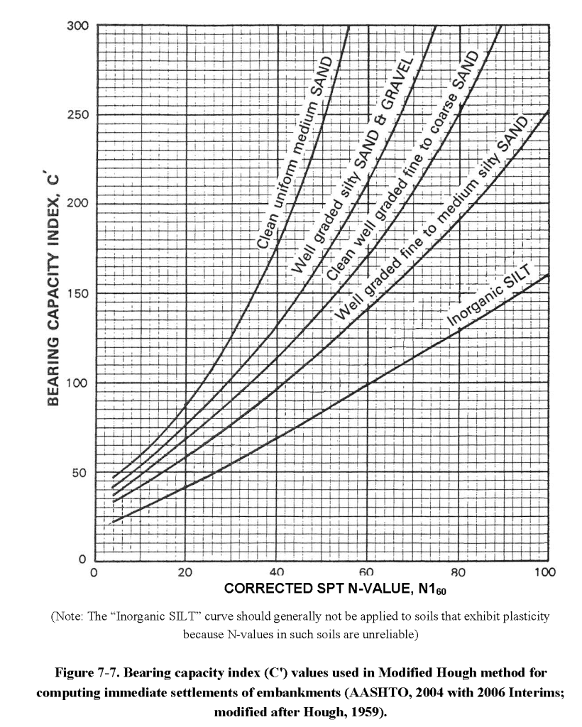
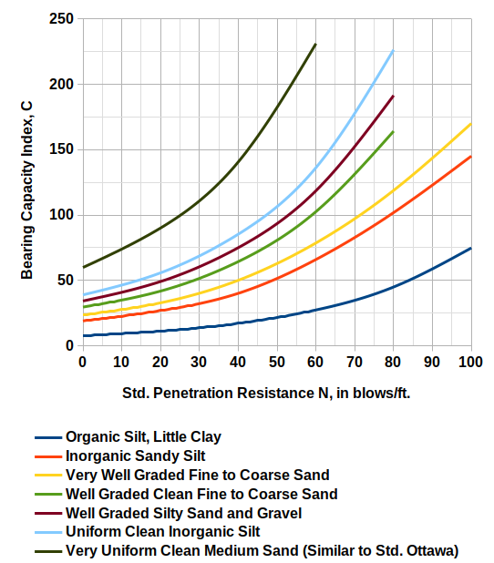
Let’s start with the first problem: the curves reproduced from the 1959 version (from the FHWA’s Soils and Foundations Manual) are here:
Figure 1 Bearing capacity index (C’) values used in Modified Hough method for computing immediate settlements of embankments (from FHWA (2006))
We’ll deal with the business of N160 shortly. There is no evidence that Hough meant to restrict his method to embankments.
The chart from the 1969 version is reproduced below (my reproduction):
Figure 2 Hough’s Method Relationship between N Values and C’ Values (redrawn from Hough (1969))
One of the more thoughtless things the FHWA has done in publishing this method is never presenting any equations for these curves, which are easily obtained using linear regression. I have done this and you can see them in Getting to the Legacy of B.K. Hough and his Settlement Method.
Obviously these sets of curves are not identical; the soil classifications he uses aren’t either, and there are five (5) curves in the 1959 version while there are seven (7) in the 1969 one.
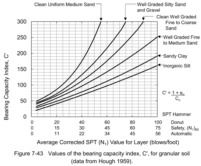
Turning to the second problem, in neither of Hough’s original monographs is any kind of correction–mechanical or overburden–are mentioned. The FHWA has consistently added overburden correction. As far as mechanical correction is concerned, in Design and Construction of Driven Pile Foundations, 2016 Edition the FHWA has assumed (not unreasonably) that Hough obtained data from a donut hammer and their correction (which also includes overburden correction) looks like this:
Figure 3 Values of the Compression Index C’ for granular soil (from FHWA (2016))
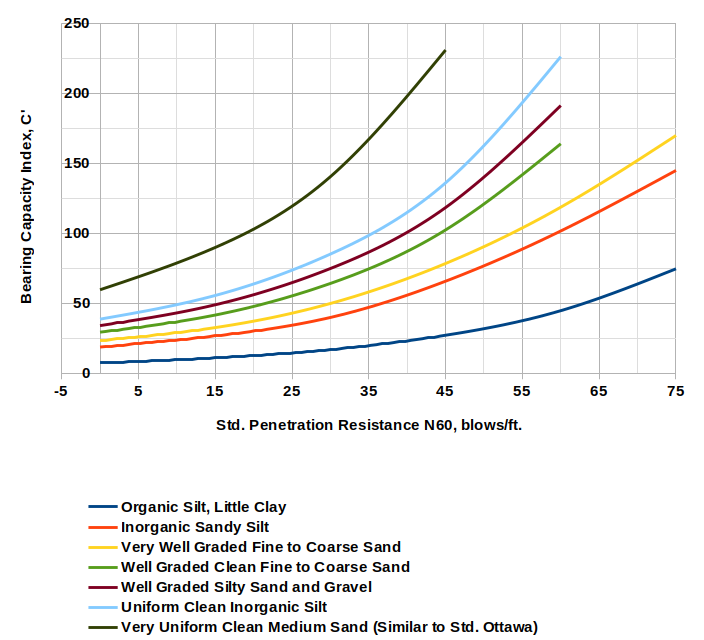
In the same vein I shifted the x-axis of Figure 2 for N60 values as shown below.
Figure 4 Relationship of N60 Values to C’ for Hough (1969) Method Assuming Original Donut Hammer
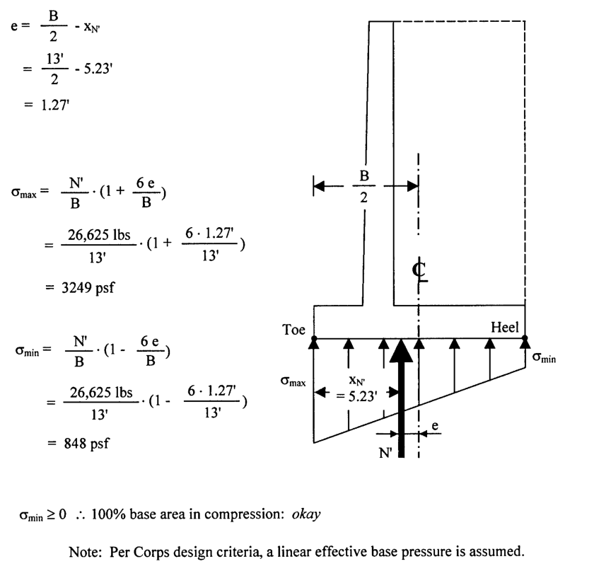
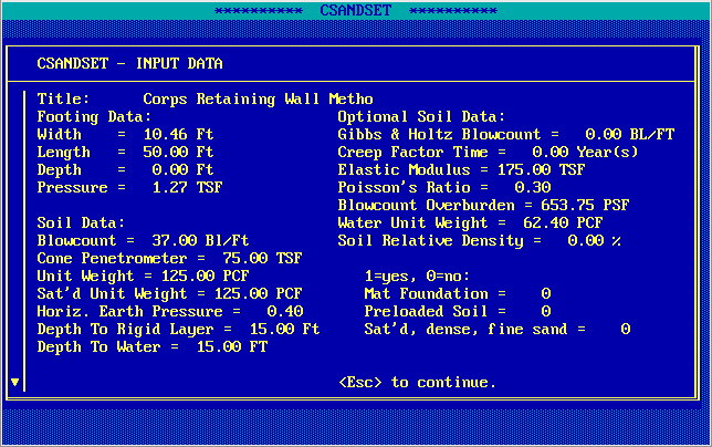
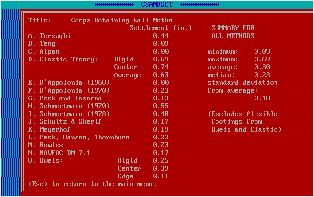
With that out of the way, the best way to illustrate the use of Hough’s Method is using a worked example, in this case a retaining wall foundation from A Simplified Method to Design Cantilever Gravity Walls. The diagram at the top of the page shows the foundation; the settlement calculations for a variety of methods (using the U.S. Army Corps of Engineers’ CSANDSET program) are given there. Let’s begin by reproducing those results below.
This program includes a fairly broad selection of methods, from elastic/theoretical ones to purely empirical ones. These methods are described in the program manual. While some of them may not be really applicable to this type of foundation, they show the wide variations of these methods, which suggests that there is not a consensus on computing these values.
Hough’s Method is not included. The detailed solution to the problem is contained in this spreadsheet. We assumed that the soil was well-graded fine to medium sand. There are four variations to the results, which are shown below:
As has been documented widely, the results of Hough’s Method are generally above most of the methods used in CSANDSET, although in the case of Schmertmann’s Method (which has been widely disseminated) the difference is not so great. The largest of the Hough’s Method variations is the Closing the Loop (or at least trying to) on Hough’s Settlement Method proposal, so I ran this with the N1(60) values, which resulted in settlements between the two FHWA methods.
One thing I would caution about using an “academic” problem as an illustration is that the parameters–many of which are taken from “typical” values–may not be representative of what actually occurs in the field, and may yield less than satisfactory results, especially for methods with a strong empirical basis. I ran into this problem with Driven Pile Design: Three Methods of Analysis. On the other hand field results are specific to their location and may not be representative of soils that the geotechnical engineer can expect to encounter.
New Values of C’
I’m not sure how much progress has been really made in this discussion. First I summarised my last two posts on Hough’s Method and how it comes up with the value of the compression constant C’, which is an alternative method of using consolidation settlement techniques to estimate one-dimensional settlement. Then I applied this to an example. Both of these have some value but they don’t get to the heart of the issue: we need more reliable (or at least values of which we understand the source) of the compression constant C’.
One hallmark of many of the fixes for this method is the invocation of overburden correction, which (as we saw above) reduces the resulting settlement. Doing this reminds me of something my Computational Fluid Dynamics I professor put in his notes many years ago:
Also, a few words need to be said about how one should interpret results ensuing from a computational simulation. There are a couple of anecdotal-based observations that are often used to describe how to approach a calculated result: (1) Computed results are guilty until proven innocent, and (2) There’s nothing more dangerous than answers that look about right. These observations are related but have slightly different interpretations. The first says that newly computed results should always be viewed with aggressive skepticism. In other words, a CFD practitioner should never accept a computed result as “truth” or representative of Mother Nature until exhaustive means have been taken to ensure that the result is a “reasonable” approximation to reality. The second observation simply means that if a calculation gives results that are orders of magnitude different from those intuitively expected, then the results can usually be quickly judged as erroneous and there is work to do to find out why. The difficult part comes when a calculation gives results that are “close” to what was expected. Such an outcome often lulls the researcher and/or practitioner into thinking that “all is well” and there is no reason to continue scrutinizing the results. However, it is very possible that a “good” answer was obtained for the wrong reason.
Compression constant typical values aren’t exactly plentiful. This table, from Verruijt, is one I have put in my course materials for many years (for log10 formulations):
Type of Soil
C’
Sand
20-200
Silt
10-50
Clay
4-40
Peat
1-10
Another tabulation comes from this source, converted to log10 values:
Soil
Minimum C’
Maximum C’
Loess silt
6.5
19.6
Clay
13.0
52.2
Silts
26.1
65.2
Medium dense and dense sands
65.2
87.0
Sand with gravel
108.7
None
Hough (1969) himself suggests another way forward. Referring to his table of compression coefficient parameters reproduced in Getting to the Legacy of B.K. Hough and his Settlement Method, we start by noting that he computes the values of Cc using the following equation:
(2)
Since the compression coefficient and constant are related in this way
(3)
we can combine these equations and compute the compression constant thus
(4)
Doing this for Hough’s values of a and b (and one should be aware of the caveats he puts on values of b) for a range of void ratios yields the following tabular result:
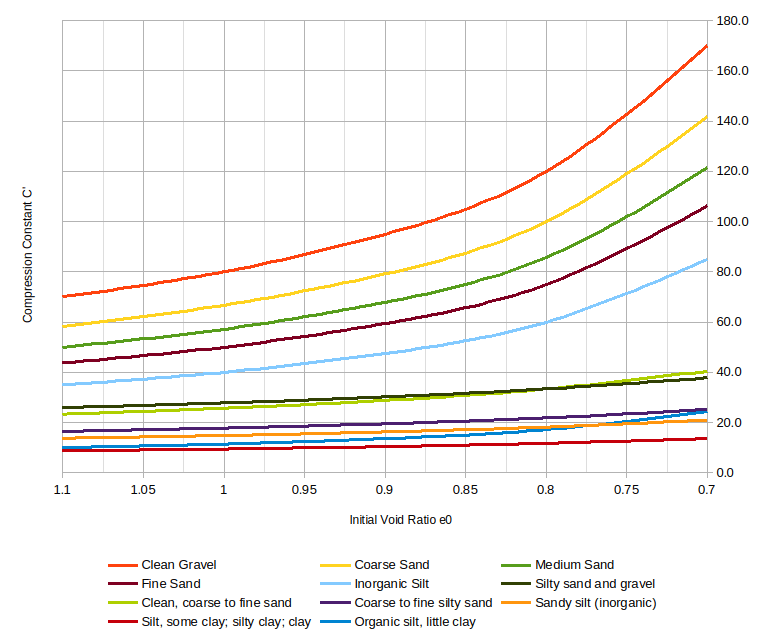
Hough’s Coefficients
Initial Void Ratio e0 (first row) Values of C’ (rows that follow)
Soil Type
a
b
1.1
1
0.9
0.8
0.7
Clean Gravel
0.05
0.5
70.0
80.0
95.0
120.0
170.0
Coarse Sand
0.06
0.5
58.3
66.7
79.2
100.0
141.7
Medium Sand
0.07
0.5
50.0
57.1
67.9
85.7
121.4
Fine Sand
0.08
0.5
43.8
50.0
59.4
75.0
106.3
Inorganic Silt
0.1
0.5
35.0
40.0
47.5
60.0
85.0
Silty sand and gravel
0.09
0.2
25.9
27.8
30.2
33.3
37.8
Clean, coarse to fine sand
0.12
0.35
23.3
25.6
28.8
33.3
40.5
Coarse to fine silty sand
0.15
0.25
16.5
17.8
19.5
21.8
25.2
Sandy silt (inorganic)
0.18
0.25
13.7
14.8
16.2
18.2
21.0
Silt, some clay; silty clay; clay
0.29
0.27
8.7
9.4
10.4
11.7
13.6
Organic silt, little clay
0.35
0.5
10.0
11.4
13.6
17.1
24.3
Graphically this is what it looks like:
Although I would be reluctant to reconstruct the method based on this, it shows one important thing: there’s more than one way to get to these constants. If we want to have a method for consolidation settlement type solutions for cohesionless soils, we need to pursue all of the following:
SPT correlations, based on current practice for correcting and applying the results.
CPT correlations. Although not appropriate in all stratigraphies (what method is?) CPT is very useful and more consistent than the SPT in those stratigraphies where it can be applied successfully.
Basic soil properties such as void ratio, relative density and unit weight. This suggests lab tests on undisturbed samples; the problem here is that getting undisturbed samples of cohesionless materials into a consolidation testing machine is easier said than done.
It’s also possible to use tests such as the pressuremeter and dilatometer, but these would only be meaningful in places where they are commonly used.
Doing all of these things would advance our understanding of the settlement of shallow foundations and give us more meaningful comparison with finite element methods.
Unlinked References
Fletcher, G.F.A. (1965) “Standard Penetration Test: Its Uses and Abuses.” Journal of the Soil Mechanics and Foundations Division : Proceedings of the American Society of Civil Engineers. Vol. 94 No. 4, pp. 67-75. It is interesting to note that Fletcher cites Hough’s First Edition of Basic Soils Engineering, while Hough (1969) cites Fletcher (1965).
Hough, B.K. (1959). “Compressibilty as the Basis for Soil Bearing Value,” Journal of the Soil Mechanics and Foundations Division, ASCE, Vol. 85, Part 2.
Hough, B.K. (1969). Basic Soils Engineering. Second Edition. New York: Ronald Press Company.
Although the inclusion of these is “obvious,” some background is in order.
When the original DM 7.01 and 7.02 were introduced, examples were scattered throughout the books, and were of variable quality, generally not very detailed. Combined with the terse (and sometimes cryptic) guidance, the lack of detailed examples made them difficult to use in an academic setting for something other than a supplement, and including more examples would have made the concepts clearer.
DM 7.01 and 7.02 came at the end of a fruitful period of knowledge expansion in geotechnical engineering, but even towards the end of the 1980’s things were happening (many documented in NAVFAC DM 7.2) that really begged for an update. With the pedagogical deficiencies noted earlier, a comprehensive teaching document was needed to educate engineers and other practitioners in the science of geotechnical engineering, and that came forth in the Soils and Foundations Reference Manual. Although many of the facts (and figures, albeit redrawn) came from DM 7.01 and 7.02, the book was structured for an educational setting, complete with worked examples (which you can see now in NAVFAC DM 7.2.) Although it was intended primarily for short courses, it could be used for undergraduate students, and (with supplements) I used it in both my Soil Mechanics and Foundation Design and Analysis courses.
It is my hope that the FHWA will revise the nearly twenty year old Soils and Foundations Reference Manual, which is complementary to these new DM 7 documents.
An Announcement About DM 7.1
This site was quick to publish NAVFAC DM 7.1 when it came out in 2022, and it has been a success. There were a few typos and places where revision was needed, and about the time NAVFAC DM 7.2 came out Change 1 to NAVFAC DM 7.1 was also released. That Change was incorporated into the print document and can now be ordered. Whether you never bought NAVFAC DM 7.1 before or just want a corrected copy, it’s available both from the publisher and now in distribution, so you can order it in places such as amazon.com.
Some Parting Observations
The whole DM 7 project, including both NAVFAC DM 7.1 and NAVFAC DM 7.2, was a monumental task. While I voiced my objections about many things, most of these were about the state of geotechnical practice and how it can be improved. As books which document the state of the practice, NAVFAC DM 7.1 and NAVFAC DM 7.2 will become necessary references.
With many thanks to the authors and all of those who worked on these books, just one thing: don’t wait so long to update it…
The last chapter (the example problems, which we plan to discuss in our last post of the series, are in an appendix) of NAVFAC DM 7.2 is on probability and reliability in engineering. Generally speaking engineers associate this with LRFD, and there have been objections to this being applied to certain geotechnical problems, as Mark Svinkin noted in his Letter Concerning Dynamic Methods. However, these methods are here to stay, and this chapter provides a comprehensive overview of the topic that goes past LRFD, which will be useful to many of the “old heads” unfamiliar with statistical methods. (Statistical methods, like linear algebra, are just about de rigeur in engineering curricula these days, not the case in the past.)
In some ways this is the best written part of the book, probably (pun partially intended) because it was written from the “ground down” (this is a geotech book, after all.) In previous chapters the authors had to wrestle with material which they felt engineers expected and whether to keep certain items or to pitch them. In this case the presentation was free of those conflicts, although the subject matter introduces complexity which can glaze the eyes.
A Basic Declaration
One thing that the chapter sets forth, in common with many presentations on the subject, is that engineers in the past have used “deterministic” methods while now we used “probabilistic” methods. This is simply not true. The factors of safety, as they lumped the uncertainties of loads and resistances into one number, may have been crude in their way of incorporating uncertainty, were in fact a recognition of uncertainty. Attempts to sort out the sources of uncertainty have been ongoing since Isaacs’ famous “factor of ignorance” statement in 1931. Beyond that, geotechs in general have been very aware of the uncertainties of designing structures in and next to the earth, which is why “engineering judgement,” not a well quantified thing in itself, has been critical in the way things get designed and built.
There are three basic problems with statistical methods.
The first is that, while the way the physics are quantified in this profession hasn’t changed (at least not enough, as I’ve noted in this series more than once) the way we deal with uncertainties has made the design process considerably more complicated. That’s why, when teaching Foundation Design and Analysis, I waited until the end to introduce Foundation Design and Analysis: AASHTO LRFD Method. It was hard enough to get the students proficient in the basic physics without adding the complexity of LRFD.
Second, NAVFAC DM 7.2 mentions the fact that some LRFD factors were based on ASD safety factors. This was very much in vogue in Geotechnical LRFD’s early years, as you can see in this document. When this fact was stated during an ASCE national convention in the late 1990’s, Jean-Louis Briaud asked the obvious question: if we’re basing load and resistance factors on ASD, what’s the point of LRFD? That question has been answered in the intervening quarter century to a large extent, but given the variations in geotechnical data (and age; I recently performed a drivability study using boring data from the 1940’s) I don’t think we’re quite there.
One thing that statistical methods are much better in doing than ASD is including the effects of “black swan” events such as earthquakes, hurricanes, and ship impacts.
Outline of the Chapter
The chapter has four main sections:
An Introduction to the topic.
Principles of Statistics and Probability, a nice overview of the basic concepts.
Uncertainty in Geotechnical Engineering, outlining the sources, effects of and designing for uncertainty.
Applications, including an overview of LRFD. The last doesn’t include a tabulation of load and resistance factors. This is doubtless a wise decision because a) there is more than one system of these, and b) they, like the tax code, have all the stability of Burnham Wood, and are subject to change by their promulgators.
One interesting inclusion of statistical methods are Monte Carlo methods, which are notoriously computationally expensive.
Overall this is an excellent section on a topic which is developing in several ways and will grow in importance in geotechnical analysis and design.


 (1)
(1)
 (2)
(2) (3)
(3) (4)
(4)