vulcanhammer.net

Some Thoughts on Changes in the Engineering Curriculum

Posted on 26 June 2026 by Don Warrington

This post has been a long time coming. I’ve been teaching engineering for a quarter century now, and when not doing that developing sites like this so that engineers (and others) can learn more about design and construction of geotechnical structures (and all structures, to varying degrees, are geotechnical unless they float on the water, in the air or in space.)

I come from a long time of technically educated people, as visiting my sites vulcanhammer.info and Chet Aero Marine will show. My great-grandfather learned the basics from Smith’s Mechanic at the University of Illinois in the 1870’s and both he and his brother had successful careers as naval architects. So I come to this debate with a long family history in this profession and many years of experience in the design and application of construction equipment, which is why my teaching straddles both Civil and Mechanical engineering. Many of those who have visited this site are familiar with my Soil Mechanics, Soil Mechanics Laboratory and Foundations courses. After teaching these for a long time, it was evident that our students weren’t “getting it” on what I thought were fundamental concepts. Moving to Lee University and teaching Statics and Dynamics only confirmed those suspicions. Added to my experience with Fluid Mechanics Laboratory and later Fluid Mechanics and this post is the sum of my reflections on this experience.

For those of you who would like a more specifically geotechnical focus, you might find my 2024 piece My Response to Rodrigo Salgado’s “Forks in the road: decisions that have shaped and will shape the teaching and practice of geotechnical engineering” and an announcement interesting.

First, let’s look at the challenges we face:

The Challenges

The growth in the use of numerical methods while the curriculum still emphasizes the use of “hand calculations.” A lot of that is driven by testing; as my CFD professor said after a disastrous midterm (and it was a 500 level course!) testing isn’t perfect but it’s the best thing we have to evaluate whether students are learning the material. The problem with this is that engineers tend to regard results that a computer produces come from Mt. Sinai (the “black box” phenomenon”) and this does not lead to good engineering practice.
We all too frequently lose sight of the fact that our first purpose is to teach people how to think, not just how to make computations or apply formulae. The latter is especially tempting in geotechnical engineering because so many of our formulae are empirical to varying degrees, but we’re not the only people with this problem.
AI, for all of its potential and actual benefits, encourages mental laziness. There, I said it. That’s the root problem with AI, and everything else only leads to that. We don’t need mental laziness in this profession or any other for that matter.
Students’ ability to visualise problems has deteriorated with the growth in computer graphics, from CAD to all kinds of 3D modeling. One thing that vanished before I got into this was students’ ability to draw, but we need to make CAD a solution rather than a problem.
Engineering curricula suffer from being squeezed into a smaller and smaller portion of the course of study engineers are required to take. State school people will recognize the fight with “GenEd” people but it’s not only a problem with state schools.

This last point is not only fueled by the amour-propre of non-STEM faculty; it comes from something that I’ve noticed over the years on Positive Infinity: there is a deep-seated fear that engineers and other scientifically trained people, without the benefit of a liberal arts education, will take over society and enforce a cold, uncultured ethic on everyone else. But that exposes one of the main weaknesses of the American educational system: we warehouse people for over a decade before expecting colleges and universities to impart to them “culture” and “critical thinking skills.” Both of these should be formed long before they step into the halls of “Old Ivy” or “Old Kudzu” (the latter is becoming more important these days.) Our biggest problem is that we cannot agree on a “culture” to teach our young people let alone whether an educational institution of any kind can or should impart such things.

Having said all that, let’s get to the concrete suggestions.

Dial Back or Lose Vector Analysis in Solid Mechanics

One of the advantages of living in the internet era is that we can easily look up books from the past, especially if they’re out of copyright. Engineering education, in a sense, is moving from the oldest knowledge to the newest, the oldest coming first in the early years and as one progresses one learns the newer stuff until, hopefully, the student meets the latest when they get the “terminal degree.” (Geotech warps this process because its transition into true scientific territory is later than other disciplines.)

Now that we have archived textbooks, we can see this process in the books that are readily available. From my great-grandfather’s Smith’s Mechanic to Analytical Mechanics for Engineers to Statics and Dynamics of a Particle, both the content and the pedagogy advance. We also have the Soviet books of a newer vintage; they had a poor economic system but an excellent educational one, and produced texts such as Theoretical Mechanics and Theoretical Mechanics: A Short Course. Other disciplines show the same trend. In all cases engineers trained under these methods went on to produce excellent designs even with the lack of computational power because they were forced to develop serious engineering judgement.

Around World War II we saw in this country a shift to a more precise and analytical approach to teaching solid mechanics. A large part of that was the application of vector analysis, especially for three dimensional problems. When I was taking these courses in the early 1970’s, one could expect to use these in practice. Today that expectation was gone; all problems but the simplest are subject to some kind of numerical method. We would be better off going back to what I call “old coot statics” and dynamics (two-dimensional analysis without vectors) and leave the three-dimensional problems to the numerical methods. Students today, especially with their visualisation problems, need to concentrate on developing their thinking skills and not get bogged down in vector analysis, which in turn is similar enough to linear algebra to develop confusion of both.

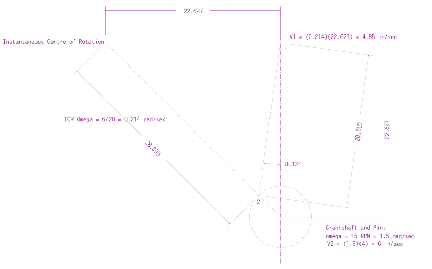
An example of the contrast between old coot statics and vector statics can be seen in the example Vector Statics and “Old Coot” Statics: An Example. In the example the two computational methods are set out side by side; the vector analysis is considerably more complicated.

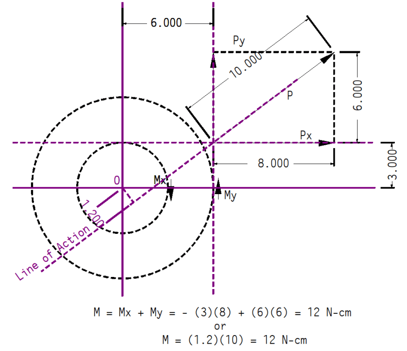
Vector analysis also obscures the fact that a moment is the product of the force and the perpendicular moment arm from the point of application to the line of action of the force. This is illustrated in An Example of 2D Moment Computation. In fact that’s the key problem to vector analysis: the student gets bogged down in setting up the problem rather than understanding its nature.

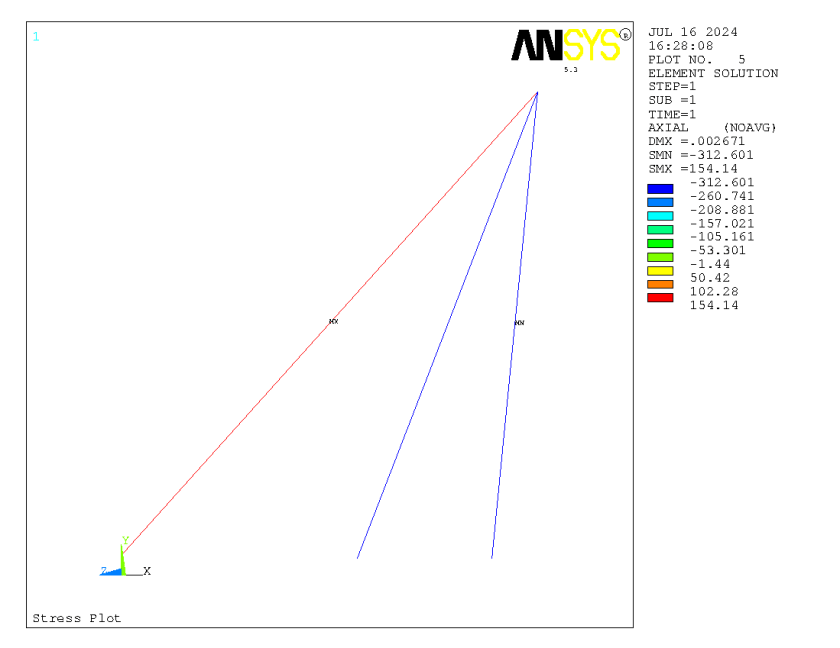
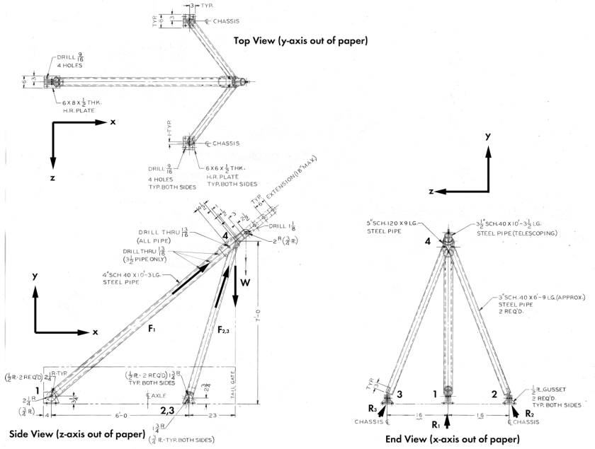
Problems–especially three-dimensional ones–are best left to numerical methods and emphasis on two-dimensional problems for basic understanding would be a better approach. The last example I’d like to give is An Example of 3D Vector Statics With a Simple Truss. Here we have a problem where (as you can see in the example itself) the vector solution is just too much for the problem; we could either a) use a numerical method or b) split the problem into two two-dimensional problems, one in the x-y plane and the other in the 2-3-4 plane.

The solution in ANSYS (I know this is an old version, we run on a low budget on this site) is below.

I’m aware that vector analysis is well embedded in the teaching of mechanics, but I think it’s time to take a serious look at the problem.

Bring Back Graphical Methods

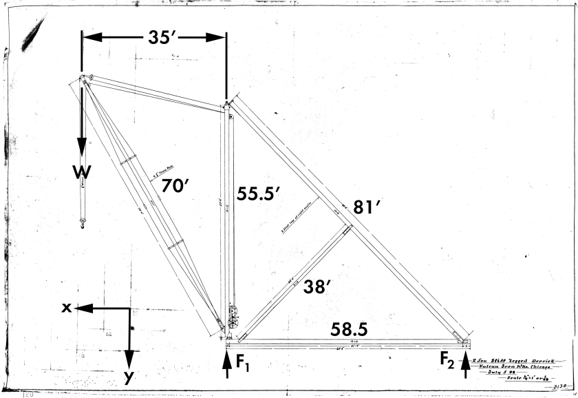
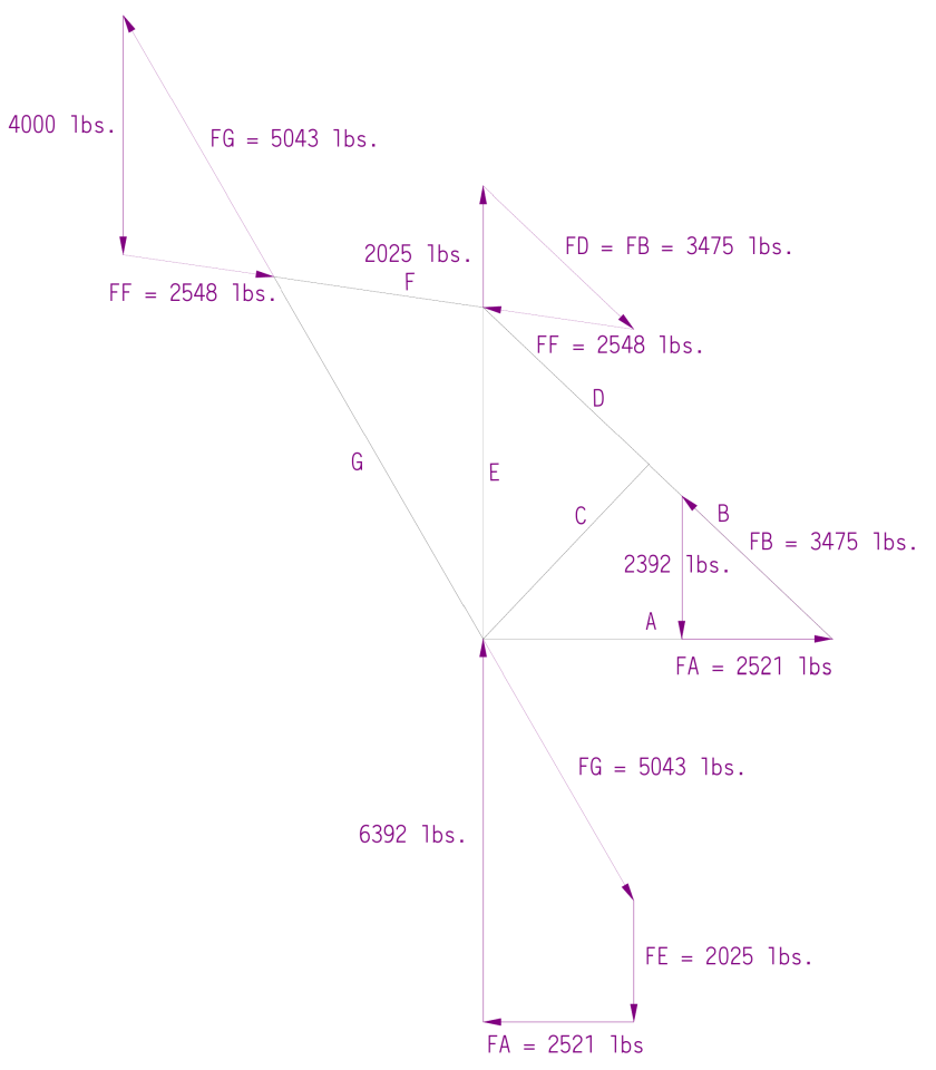
One hallmark of engineering practice in the past was the use of graphical methods to resolve forces and perform other tasks which would be computationally expensive. The advent of the calculator and later the computer into the profession gave the impression that graphical methods were a thing of the past.

With CAD that’s not the case: we can solve problems with the same precision in CAD we do with either vector analysis or “old coot” statics. An example of this comes from the very first example shown; the graphical solution is given in the article Stiff Leg Derrick Part II: Truss Analysis, and can be seen below. The magnitudes were measured in CAD and the directions were done using the basic derrick layout in CAD.

Another example of a semi-graphical method that gets the short shrift these days is rotation about an instantaneous centre; I give an example of this in Solving a Dynamics Problem using the Instantaneous Centre of Rotation with a Vulcan Design.

Graphical methods will assist visualisation and give students a better feel for the problem, both of which they need in their development as engineers.

Distributed Loads and Concentrated Resultants

This comes out of my geotech teaching but also Fluid Mechanics as well: my students struggled with the transition from distributed loads to concentrated resultants. And the distributions were the usual ones we see in geotech and Fluid Mechanics: linear, either uniform, triangular, or trapezoidal. I’m not sure what the solution is but there are two things we need to consider: a) the aforementioned vector statics and b) the inclusion of algebraically complex loadings with polynomial or other higher order equations. As a practical matter it’s unlikely that a complex loading encountered in practice will obey these equations but will more likely require a stepped type of loading of some kind, which in turn begs a numerical solution.

Keep Basic Fluid Mechanics Basic

Fluid Mechanics has experienced much of the same transition as solid mechanics. From books like Hydraulics and Fluid Mechanics to those we usually teach from now, an emphasis on practical fluid mechanics has been lost. In my own career I have found that many of the problems I had would have been much easier to see if the curriculum I was taught under had stuck with a more basic approach (and books which emphasise that do exist, as you can see from my own course.) What we need is to do the following: a) save much of the more theoretical treatment for an advanced course, paralleling that of mechanics of materials, and b) integrating that type of material into basic Computational Fluid Dynamics, which is a necessity for many fluid mechanics problems.

One other thing worth mentioning is that, in the past, solid and fluid mechanics were more integrated, as you can see in books from Smith’s Mechanic to Mechanics by S.P. Strelkov. We might consider some of this if we decide to seriously rearrange how we teach these subjects.

Putting a Wrap

This is not meant to be an all-inclusive list, and I realise that some of these suggestions will be controversial. Today it’s fashionable in higher education, as it has been down the line for many years, to emphasise the pedagogy methods as opposed to the content. But a simpler, more straightforward approach to subject would lend itself to easier pedagogy; the two aren’t unrelated. The tendency to push practitioners out out teaching–one driven in part by our accreditation process–has left many with an unclear understanding of what is required of engineers once they graduate. There are many issues we face; this piece is only meant to start the conversation, not finish it.

Location of Corner of Failure Envelope for Anchored Sheet Pile Walls

Posted on 1 May 2026 by Don Warrington

A recent inquiry revealed that the literature on this site and vulcanhammer.info has a difference of design procedure for anchored sheet pile walls.

In order for a deadman anchor to be effective, it must be beyond the failure envelope. Here we present two ways to insure that this is so.

The first is shown above: it is taken from NAVFAC DM 7.2, although it has been in many publications over the years, including NAVFAC DM 7.02 and Sheet Pile Design by Pile Buck. It shows the point at which the failure envelope starts as the “estimated point of zero moment in wall.” That can be determined using software such as SPW 911.

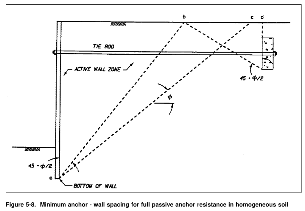
The second is shown below, from EM 1110-2-2504, and shows the same point at the bottom of the wall.

If you have any comments about either of these methods, or which one you prefer and why, let us know in the comments.

Geotechnical Engineering, Deep Foundations

Comments on “Inverse analysis for parameter estimation of sandy soil with axially loaded pile using nonlinear programming”

Posted on 16 January 2026 by Don Warrington

This is yet another commentary on a paper which cites my work, in this case Inverse analysis for parameter estimation of sandy soil with axially loaded pile using nonlinear programming, which cites Improved Methods for Forward and Inverse Solution of the Wave Equation for Piles. Since 2026 is the tenth anniversary of the publication of that effort, some remarks on why I did that are in order.

Rationale for My Original Study

The current predominant regime in pile dynamics has been around for over half a century now. With tweaks and improvements in computer power and hardware, it has enabled us (well, most of us) to jettison the problematic dynamic formulae for capacity prediction and verification during installation. The whole system, however, relies on the 1D representation of pile/soil interaction to be accurate and the optimization algorithm to find the solution to the inverse problem. Both of these are subject to the kinds of improvements we see in other fields.

Getting to this point was not an easy or straightforward task, both because of the application itself and the code/regulatory environment in which we operate. Much of the struggle to get the current methodology accepted was an uphill battle against the existing “we’ve always done it this way” mentality which settles in, and no doubt this will be the case with a new generation of pile dynamics methodology. But there are some difficult challenges inherent in the physics of this problem, most of which stem from the nature of soils themselves.

I ran into many of these challenges during my study which led to Improved Methods for Forward and Inverse Solution of the Wave Equation for Piles. One colleague from an institution in a neighbouring state felt that my effort was “too ambitious.” He’s probably right, which is why he’s in administration now. But my objective was for this study–and the subsequent papers to fine tune the method–to be a convesation starter, and this paper’s citation of my work is evidence that this is taking place. I sense that efforts to “move the football down the field” in this discipline are taking place, and am gratified to be a part of that effort.

Comments on the Paper Itself

Strictly speaking this paper only has the inverse method as a commonality with my own study. In this case the researchers are dealing with a drilled shaft and are trying to back analyse static capacity. While this sidesteps the rate-dependent problem between dynamic signals and static response, it brings other factors into play, some of which are definite weaknesses in the paper and others where the jury is still out.

Optimisation Technique

Let’s start with one which falls into the latter category: the optimisation technique they chose, which was the Davidon-Fletcher-Powell method. The purpose of optimisation techniques is to find the minima and maxima of “equations” (often they can be expressed in this way, but in this business frequently they can’t) and thus the best solution to the problem. The classic example of this (and one frequently used to test optimisation techniques) is the Rosenbrock Equation, which is

$z = (a-x)^2 + b (y-x^2)^2$

and is plotted as shown below for a =1 and b = 100.

This has challenged optimisation techniques for a long time. The problem with using something aimed at problems like this is that, in geotechnical engineering, problems look less like this and more like relief maps. The result is having to deal with false minima. For example, if we have a canyon on top of a plateau, a false minimum would be the lowest elevation at the bottom of the canyon rather than the bottom of the cliffs of the plateau, which are generally lower. Multiple false minima are common for problems in this profession, which is one reason why we still use brute force grid optimisation in problems like slope stability. This is why I chose a polytope method for my own study, which is derivative free and “casts a wider net” on the downhill slopes of a problem. It is slow and its results not perfect but I think this is a problem that needs to be addressed if we are to use optimisation techniques for solving geotechinical problems.

A couple of side notes:

I did use a quasi-Newton routine related to the DFP method in my study “Analysis of Vibratory Pile Drivers using Longitudinal and Rotational Oscillations with a Purely Plastic Soil Model” because I felt the parameters were “regular” enough to justify its use. The routine I used had an option for the BFGS (Broyden–Fletcher–Goldfarb–Shanno) method. And that leads to…
My last course for my PhD degree was in Optimisation. One day our professor–Dr. Kyle Anderson, one of the most brilliant people I’ve come to know–was going on about these techniques, and as you can see Roger Fletcher’s name comes up in many of them. So I leaned over to one of my classmates and said, “Fletcher sure does play both sides of the street.” Dr. Anderson was irritated at seeing whispering, and made me repeat this to the whole class. When I did he thought for a second and said, “He does play both sides of the street.”

The Capacity Issue

In the paper at hand, the optimisation technique starts with initial values and comes to back-analysed values which are then compared to reference values. The problem here is that the reference values are based on single values of toe capacity and soil parameters, the latter of which are related to static methods of analysis. There are two problems which arise in this approach.

The first is the variability of static methods relative to the actual performance of the deep foundation. This is evidenced by the wide scatter in the results these methods return (it’s not quite as bad with drilled shafts as it is with driven piles, but it’s bad enough.)

The second is that the whole business of the “capacity” of deep foundations–ultimate, allowable or factored–cannot be divorced from the fact that the resistance of piles to load takes place through a distance, or settlement. Capacity doesn’t mean much when it’s decoupled from settlement. For static analysis the Holy Grail needs to be that we can estimate the distribution of pile resistance–both between the shaft and the toe and along the shaft–from static load tests. Using static “capacities” may have made the optimisation method they chose possible to use but it does not really get us to where we need to go. Dynamic testing and methods such as CAPWAP recognise this problem but, as noted earlier, improvements there are possible if not easy to arrive at.

Conclusion

I think this paper is an interesting study as a step towards using optimisation techniques to solve the inverse problem of pile resistance to axial load. But there are many more issues to deal with if we are to come to a workable solution for this problem.

Deep Foundations, Soil Mechanics

Comments on “Using the Impulse-Response Pile Data for Soil Characterization”

Posted on 15 January 2026 by Don Warrington

This is another post on a paper (linked to from here) which cites my work, in this case two of them: Improved Methods for Forward and Inverse Solution of the Wave Equation for Piles and Closed Form Solution of the Wave Equation for Piles. The concept is simple but the execution, not so much, and as with anything with geotechnical engineering there are pitfalls on the way to a usable solution.

We start with an existing technology: low-strain integrity testing of piles. A simple example of this is shown above, it’s the Pilewave program from Piletest. (Yes, I’m aware that it’s the Windows 3.1 version, if you’re interesting in running DOS and Windows 3.1 programs to save on the expense of “new” engineering software, you can visit Partying Like It’s 1987: Running WEAP87 and SPILE (and other programs) on DOSBox.)

With that distraction out of the way, note that, as the stress wave goes down and back up the pile, there is attenuation due to the interaction with the soil. In the simple demo of Pilewave, the soil resistance is constant along the shaft. But…if we could determine that the pile didn’t have defects which reflected waves, could we use information from the soil attenuation to determine the type of soil surrounding the pile at any given elevation? The answer in principle is “yes” and this paper, although not unique, it is an interesting step forward.

Pile Integrity Testing is a low-strain technique. That’s in contrast to the high-strain methods we’re used to in pile driving analysis. This one takes a leaf from the seismic refraction method (which will be featured as before in Soils in Construction, Seventh Edition) which is also a low-strain technique, as it is a geophysical method. The idea is that the pile acts as a probe into the soil; the response to exitation can be inversely analysed to determine the types of soils around the pile. As the paper notes, if you divide up the pile into enough “layers” the actual soil layering itself (based on the properties returned to you by the method) will basically emerge from the data.

As is generally the case with inverse methods, the solution is complex; it is described in the paper. There are a few comments that I would like to make as follows:

His governing equations are similar to the Telegrapher’s Equation used in Closed Form Solution of the Wave Equation for Piles and include a strain term but lack a damping term. Usually a damping term is necessary to model the energy dissapation into the soil; whether that applies to this problem remains to be seen.
The toe model he used was inspired by Closed Form Solution of the Wave Equation for Piles, which I discussed relative to its origins and influence by Alain Holeyman in my recent post Comments on “Nonlinear fictitious-soil pile model for pile high-strain dynamic analysis” and “Fictitious soil pile model for dynamic analysis of pipe piles under high strain conditions.”
Driven piles are subject to compaction and disturbance at the soil-pile interface; how this affects the results remains to be seen. The difference in soil response based on rate effects also will need to be addressed.

I hope that this research continues; I think it has potential.

Civil Engineering, Soil Mechanics

New Year, New Prices: Geotechnical Books Update

Posted on 1 January 202627 December 2025 by Don Warrington

As we begin a new year (for this site, it’s the 29th) we need to clarify some things that have changed regarding our book offerings.

We’ve been with Lulu publishers since 2006 (this is our twentieth year with them) and we’ve been through many changes in the publishing industry since that time. In those days we not only offered print books (our government doesn’t print their geotechnical publications any more) but also CD’s with documents. They only sold these books and CD’s on their own website.

Later they began to offer to put books “in distribution,” i.e. with places such as Amazon.com and other book sellers. We’ve been migrating our product line in that direction but have run into two problems.

The first is that distribution is expensive; these people like to take a substantial cut. This forced us to price things accordingly, although we’ve tried to keep our own cut at a reasonable level.

The second is that the requirements for a book to be in distribution changes, or more accurately the way that Lulu and these publishers enforce these requirements changes. The result is that books which have been in distribution for years are no longer there, although they’re still available from Lulu.

Our response to this is to simply keep the books in distribution which are most popular and to allow the rest still being published to stay on Lulu. The result of that is below, with our entire geotechnical book line listed. In taking books out of distribution we’ve looked at our pricing and have reduced prices on several titles.

We’d like to wish everyone who visits this site a Happy and Prosperous New Year.