The Sorry State of Compression Coefficients

I’ve dealt with the issue of consolidation extensively since my first post on the subject, From Elasticity to Consolidation Settlement: Resolving the Issue of Jean-Louis Briaud’s “Pet Peeve”. His problem was the lack of relationship between the way we handle consolidation settlement vs. elastic settlement. In this post I plan to look at a different problem, i.e. the way we express the relationship between soil pressure and consolidation settlement, or settlement by rearrangement of the particles.

Up to now…

Let’s start with the diagram at the right, from Broms (as will be the case with the graphics we use.) Soil is made up of a combination of soil particles and voids between them. The voids can be filled with air, water or (God forbid) something else. For saturated soils water, for practical purposes, fills all of the voids.

In any case, for illustrative purposes we can “melt” the solids into a continuous solid and leave the rest as a void. We assume that the solids do not compress during the application of pressure and thus their volume is constant. From the first state (on the left) to the second state (on the right) additional pressure is applied. All the change of the volume must take place in the void; the equation at the bottom is based purely on the geometry, where $H_o$ is the height of the layer being compressed, $e_o$ is the initial void ratio of the soil, $\Delta e$ is the change in void ratio during compression, and $\delta_p$ is the primary settlement of the soil.

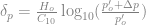
Unfortunately, as discussed elsewhere on this site, the relationship between the increase in pressure and the settlement/change in the volume of the voids isn’t linear but (empirically) logarithmic. That is shown in the graphic on the left; once the pressures get past the ambient effective stress, the settlement takes places according to the relationship shown at the bottom of the graphic. Here $C_c$ is the compression coefficient, $p'_o$ is the effective stress, and $\Delta p$ is the change in pressure on the soil at a given point.

Combining the two equations in the two graphics yields the “accepted” form of the consolidation settlement equation for normally consolidated soils, thus

$\delta_p = \frac{C_c H_o}{1+e_o} \log_{10} (\frac{p'_o + \Delta p}{p'_o})$ (1)

To this deceptively absolute state of affairs Verruijt has the following objections:

We should be using natural logarithms instead of common ones. Common logarithms date from the days when engineers used logarithmic and semi-logarithmic paper, determining $C_c$ graphically. The compression coefficients would be changed by multiplying or dividing (depending on the form, more on that shortly) by a factor of 2.3. In an era of spreadsheets and MATLAB, natural logarithms would make more sense (and reduce student mistakes,) but I don’t see that changing.
We should use the strain rather than the void ratio. Actually, as Verruijt points out, this is done in Continental Europe. In the U.S. and Scandinavia, void ratio is used as the parameter of deflection. To change this would require a change in the compression coefficient, and that leads to…
…his preferred form of the compression equation, which would look like

$\epsilon = \frac{1}{C_{10}} \log_{10} (\frac{p'_o + \Delta p}{p'_o})$ (2)

where $C_{10}$ is another form of the compression coefficient. (Well, actually, he’d prefer natural logarithms, but as I said let’s put that aside.)

Multiplying both sides of Equation (2) by $H_o$ gives us

$\delta_p = \frac{H_o}{C_{10}} \log_{10} (\frac{p'_o + \Delta p}{p'_o})$ (3)

The two compression coefficients are related as follows:

$\frac{1}{C_{10}} = \frac{C_c}{1+e_o}$ (4)

Actually a variant of Equation (4) finds its way into American practice in Hough’s Method for sands, which is described in the Soils and Foundations Reference Manual.

Enter NAVFAC DM 7.1

The “New” NAVFAC DM 7.1 (Soil Mechanics) is an excellent compendium of the current state of geotechnical practice relating to soil mechanics. In the process of discussing consolidation settlement, it highlights some recent changes that promise to add to the confusion described above.

For normally consolidated soils, Equations (1) and (3) are written as follows

$\delta_p = C_{\epsilon c} H_o \log_{10} (\frac{p'_o + \Delta p}{p'_o})$ (5)

where $C_{\epsilon c}$ is the modified compression index. This means that Equation (4) can be expanded as follows:

$\frac{1}{C_{10}} = \frac{C_c}{1+e_o} = C_{\epsilon c}$ (6)

Whether we can dispense with the initial void ratio is a separate topic. Assuming that we can, what we have is a situation with three different compression coefficients, all designated with some form of $C_x$ , and none of them the same. (If we threw in natural logarithms, we’d have six.) The potential for confusion is evident, no where than when two of the three coefficients end up in the same table:

And Secondary Compression…

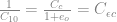
Secondary compression has had the problem for much longer. If we look at Graphic 3 on the right, we see that we have a secondary compression coefficient $C_{\alpha}$ . The presentation is a little hard to follow but the secondary compression equation is

$\delta_s = \frac{C_{\alpha}H_o}{1+e_o} \log_{10}\frac{t_{life}}{t_{100}}$ (7)

where $\delta_s$ is the amount of secondary compression, $C_{\alpha}$ is the coefficient of secondary compression, $t_{life}$ is the life of the structure and $t_{100}$ is the time at which 100% of primary compression has taken place. (Of course that’s a source of confusion in itself because, in theory, 100% primary compression is never achieved, something that buffaloed many of my students on a test last semester.)

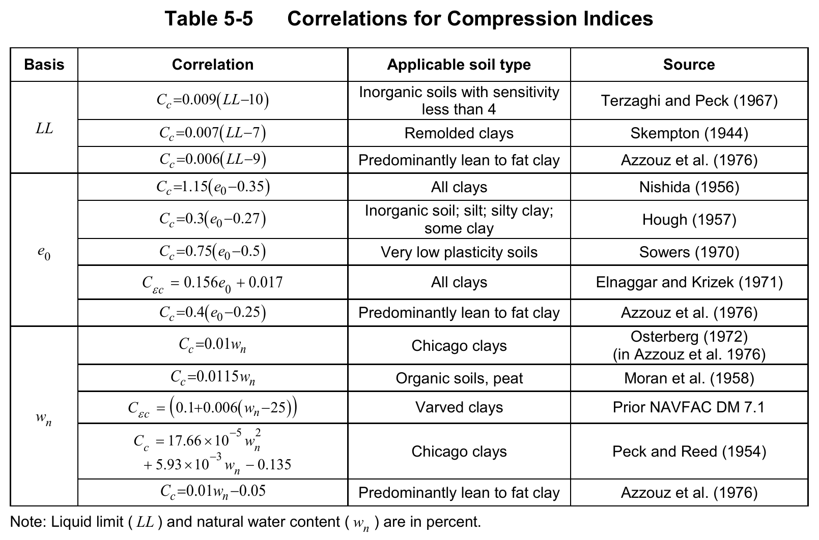
However, as NAVFAC DM 7.1 points out, we can also write this as

$\delta_s = C_{e \alpha}H_o \log_{10}\frac{t_{life}}{t_{100}}$ (8)

where the modified secondary compression coefficient is

$C_{e \alpha} = \frac{C_{\alpha}H_o}{1+e_o}$ (9)

So what is to be done?

My advise to students and practitioners alike is to be vigilant and careful. Make sure you understand which coefficient is being called for. For software, make sure you completely understand which coefficient is being used by the software; otherwise, you will have the classic “garbage in/garbage out” result. Verruijt hoped that we would come to uniform practice but we can’t wait for this; we have to get our work done, and we need to do it carefully.