Category: Deep Foundations

In our last post we discussed the origins and use of these programs to simulate–in forward or inverse analysis mode–the load-settlement characteristics of deep foundations, including driven piles and drilled shafts. In this post we will consider the potential by having these tools at our disposal and some thoughts on how to expand their use and improve their capabilities.

Bearing Capacity and Settlement

I discuss this issue in more detail in my post Driven Pile Design: Axial Loads, General Considerations (and the same considerations apply to bored piles as well.) In that post I state the following:

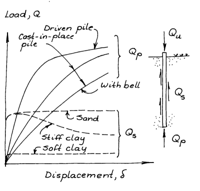
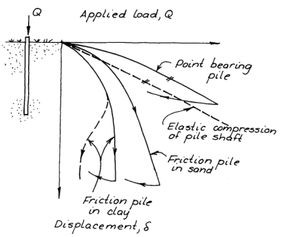
The failure of a deep foundation is progressive, as can be seen at the right. It is very seldom (unless something has gone very wrong somewhere) that pile foundations experience “plunging” (catastrophic) failure, especially if the resistance at the toe is substantial. Put in terms of engineering practice, failure of a deep foundation is most likely to be a service (settlement) failure rather than a strength (bearing capacity) failure. It thus would make sense to design deep foundations based on a settlement criterion. What settlement is acceptable depends upon the application and structure.

From this, the behaviour of a deep foundation cannot be characterised by a single number. There is a mathematical reason for that. Consider the idealised load-settlement curves below, which include a Davisson method type offset line.

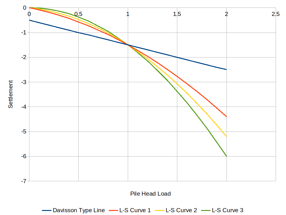
All of the curves (the units were simplified to make the curve constructions easier) pass through the Davisson failure point of (1, -1.5.) But the curves are different, albeit in this case parabolically constructed, and not only that there are an infinite number of them. Thus the load-settlement of a given single-number “bearing capacity” is not unique; the behaviour of the pile under load cannot be adequately characterised by one number.

There are other possible uses for this reality which we will discuss below. Unfortunately the introduction of LRFD has only made the situation worse by formally separating the strength (“bearing capacity”) and service (“settlement”) loads, each with their different load and resistance factor, but each with a single number.

A more sensible way of dealing with this problem would be the following:

• Determine the load-settlement curve(s) for a given project and pile/shaft configuration using software such as APILE.
• Determine the permissible settlement for a foundation depending upon what type of structure supports it. I discuss this on an elementary level in Foundation Design and Analysis: Shallow Foundations, Settlement.
• Adjust the design (or redesign altogether) the foundation until it meets with the requirements of the load. At this point it is legitimate to compare those requirements with whatever static load test capacity method is fashionable in your area, as we would compare both the pile head load and the settlement with those results. (For an overview of Davisson’s method, the most common in the US, visit Driven Pile Design: Static Load Testing and Axial Settlement.)

Since we have the tools for the first analysis, we can proceed with this method with existing technology. The major challenge is to change the design procedures, generally enshrined in the codes or job requirements, and to educate engineers in this methodology.

TZPILE and Resistance/Capacity Distribution

In the last post, we looked at TZPILE and how one could, by matching it to the load-settlement curve, construct a distribution of shaft and toe resistance/capacity along the embedded length of the pile. One is reminded of using the wave equation program to back analyse driven pile results, but these days the most common method is CAPWAP and its progeny. With the numerical methods we have at our disposal, shouldn’t it be possible to construct a distribution of resistance using static data just as CAPWAP does with dynamic?

To start the discussion, take a look at the graph above. Each of the curves (excluding the Davisson type line) represents a different combination of pile configuration and soil resistance/capacity distributions which produce the same Davisson capacity. If we fix the pile configuration, we’re left with soil variations, examples of some of which are at the right. TZPILE enables the user to match this manually. In principle we could automate the process as was done with CAPWAP.

There are, however, a few complications along the way. The math isn’t that complicated but the concepts are not in the daily currency of most practicing geotechnical engineers. I would urge you to take a look at my monograph Least Squares Analysis and Curve Fitting for the basics; it relates the topic to spreadsheet trend lines, which most are familiar with.

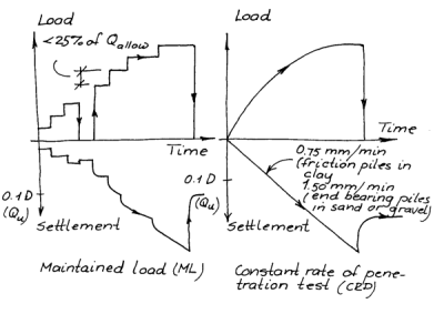
Most static load tests (in the U.S. at least) are performed incrementally, i.e., a load is applied, a settlement is reached, and another load is applied. In many cases the number of loads applied is relatively small. When it’s all done some kind of line is drawn through (or nearly so) the loads to produce a load-settlement curve.

If we do an interpolation, whether it is piecewise linear, Lagrangian or cubic spline, the only thing we can say with confidence is that the curve passes through all of the points. What happens between those point can look good or be accurate but doesn’t have to be either one; it just has to pass through the points.

If we have more or fewer data points than an interpolation would require, we end up looking not for the right solution but the best solution to the problem. That’s where Least Squares Analysis and Curve Fitting comes in, using the ||r||₂ norm. (Interestingly CAPWAP uses the ||r||₁ norm.) The coefficient of determination R² gives us a idea as to how good a fit we have, although you need to look at your results to make sure the fit makes sense.

In both cases we cannot use whatever curves between the data points we generate to “fill in” and produce enough data points to effect a one-on-one and onto linear transformation between the static load data and the number of layers the pile might be penetrating into, which is the ideal. With a small number of test loads this could lead to layers and variations in resistance being missed. This is an advantage of CAPWAP; it obtains a large number of data points during driving that in part compensate for the problems of getting a static resistance/capacity out of a dynamic test.

The problem of few load test points is an important one and an obstacle to using a program such as TZPILE on a widespread basis to estimate the load distribution on a deep foundation. If we could increase the number of test points on at least major projects and couple it with a repeatable method of determining the distribution from the load points, we would have yet another source of verification for the load-settlement characteristics of deep foundations.

In the process of doing drivability studies for Pile Hammer Equipment, I’ve noticed that some of them include use of the APILE program. APILE is a program from Ensoft, Inc., which estimates the load-settlement curve of a deep foundation. Although it was originally developed for driven piles, it can also be applied to drilled shafts and other bored piles as well. It’s been around for a while but this brief series of posts will look at two things:

• The origins and antecedents of APILE and related programs (this post)
• The possibilities of expanding the use of APILE and related programs.

APILE: The Basics

According to its description sheet, APILE’s purpose is as follows:

APILE is used to compute the axial capacity, as a function of depth, of a driven pile in clay, sand, or mixed-soil profiles.

It isn’t the first program to accomplish this; on our companion site we have featured two programs for this purpose:

• SPILE, a DOS program developed to estimate the axial capacity of piles using the FHWA’s favoured methods as described in the Soils and Foundations Reference Manual
• DRIVEN, a Windows XP-era program for the same purpose as SPILE and using the same basic methods. This was used in tandem with GRLWEAP and eventually a cut-down version of the program was incorporated into GRLWEAP.

Both of these programs were useful but suffer from two limitations:

• The operating systems are obsolete, although with SPILE that can be gotten around with DOSBOX.
• Both of these are restricted to the FHWA Nordlund/Tomlinson methods. The current version of APILE includes the following:

Several methods are used by APILE for computations of pile capacity: i) American Petroleum Institute (API RP-2A), ii) U.S. Army Corps of Engineers (USACE), iii) U.S. Federal Highway Administration (FHWA), and the iv) revised Lambda method.

The Offshore version features several more. It’s unfortunate that the Fellenius method–which is also an FHWA recommended method, albeit not its favourite–isn’t included, although perhaps it could be in a future version. It’s also unfortunate that the company that Lymon Reese started didn’t include the method developed by Reese’s long-time colleague at the University of Texas, Roy Olson, the Dennis and Olson method.

APILE also has the capability of doing the following:

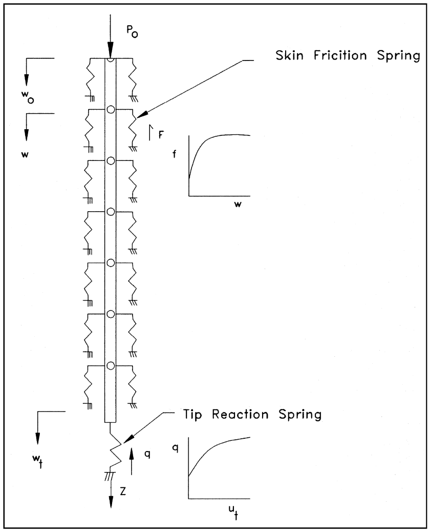
A short-term, load-settlement curve is generated for the modeled pile using nonlinear soil models and elastic pile material deformation. The APILE program uses two sets of internally generated t-z curves (load-transfer in axial side resistance as function of movement) and Q-w curves (load-transfer in end bearing as function of movement) for developing the load-settlement predictions.

The rudiments of the t-z method (which is the basis of this capability) are discussed here. What this amounts to in simple terms is performing a static load test in the computer, much as the wave equation analysis is used to predict pile behaviour during driving. That leads to the thought that one could use static load tests to determine the distribution of resistance and capacity along the pile shaft and at the pile toe. We’ll get into more detail on that in the subsequent post on APILE but there is a partial solution that is related to APILE, namely TZPILE.

TZPILE

The description sheet for TZPILE gives the following overview:

TZPILE implements the well-known method of soil-structure interaction, commonly called the t-z method, where t-z and Q-w curves are used respectively for load transfers in side resistance and end bearing. The t-z and Q-w curves can be internally-generated for both driven piles and drilled shafts with the input of information on the supporting soil and on the geometry of the pile.

The program can be used as follows:

Curves of short-term settlement as a function of applied loads are essential for some engineering computations; for example, when refined input is needed for the analysis of piles in a group. If a field-load test is performed, the computed curves can be “calibrated” by modifying input information to TZPILE to reach agreement with the experimental curves. The calibrated, site-specific curves can then be used with TZPILE to design the production piles, which may vary from the test piles in geometry and stiffness.

TZPILE is thus intended to perform the reverse task of APILE, i.e., given the results of a static load test, the load-settlement curve is matched and the distribution of resistance along the pile shaft and at the toe is estimated.

So where do these two programs come from? Based on the fact that the two were commercialised when Lymon Reese was still alive and active, it makes sense that, like WEAP and its progeny, the method had its genesis in government developed code. That suspicion was confirmed for me when I saw the text output for a pre-COVID version of APILE, which looked very much like the PX4C3 program which has been featured on this and our companion sites for a long time. So let’s take a look at that effort.

PX4C3

The description for that program is as follows:

PX4C3 is a finite difference program used to compute load settlement characteristics on an axially loaded pile of constant outside diameter. A set of load transfer curves along the pile (i.e., skin friction developed on the side of the pile relative to the absolute axial displacement of the pile section) & four point resistance curve at the pile tip (i.e., relationship between the total axial soil resistance on the base of the pile tip & the pile tip movement) are used in program to obtain non-linear soil-pile relationships. Finite difference equations are used to achieve compatibility between pile displacement & load transfer along the pile & between soil resistance & load transfer along the tip of the pile. A complete description of the program can be found in the document “Background Theory and Documentation of Five University of Texas Soil-Structure Interaction Computer Programs,” Miscellaneous Paper K-75-2, by N. Radhakrishnan and F. Parker.

At the top of the code is the following:

C WRITTEN BY H. COLE & L. REESE, U. OF TEXAS
C COMPUTES LOAD SETTLEMENT CHARACTERISTICS OF AN AXIALLY LOADED PILE
C
C 'LOAD VS SETTLEMENT FOR AXIALLY LOADED PILE'L.REESE,SYMP ON BEAR-
C ING CAPACITY OF PILES ,CNTRL BLDG RES INST,ROORKEE,INDIA,1964.
C 'UNIV OF TEXAS SOIL-STRUCTURE INTERACTION PROGRAMS'RADHAKRISHNAN &
C PARKER,WES,MISC.PAPER TO BE RELEASED 12-73.
C CONTACT N RADHAKRISHNAN OR F. PARKER, WES, VICKSBURG, MISS.
C************************************************************
C -PROGRAM USES THE GIVEN LOAD TRANSFER VS PILE MOVEMENT
C-----CURVES AND COMPUTES THE LOAD SETTLEMENT CHARACTERISTICS OF AN
C-----AXIALLY LOADED PILE
C-----LOAD TRANSFER VS PILE MOVEMENT CURVE IS DESIGNATED AS P-Z CURVE
C---PX4C3 INTERPOLATES POINT BEARING VALUES CORRESPONDING TO A GIVEN
C-----TIP MOVEMENT FROM A PREVIOUSLY INPUT POINT BEARING VS TIP MOVEMENT
C-----CURVE

The only thing that needs correction is that Reese’s co-author of the code, “H. Cole,” is in fact Harry Coyle of Texas A&M University. Evidently Radhakrishnan and Parker’s paper took longer to get “out the door” than they thought it would; the report is initially dated May 1975 (a year and a half after the date given in the code) and this was marked out on the report to July 1979, although the report described not one but five programs, one of which is the ancestor of the COM624 lateral load code which was developed both by the Corps and the FHWA and is the basis for LPILE.

APILE1

No history of this program “family” would be complete without the inclusion of APILE1. This program was used for the 1988 master’s thesis of Ronald Ungaro at Texas A&M entitled “Development of Design Parameters for H-Piles in Sand Using Static Analysis.” Ungaro, working under Harry Coyle’s direction, referenced this program as “Coyle, H.M., Marine Foundation Engineering, Unpublished class notes, Texas A&M University, Spring, 1987.” It’s reasonable to assume that Coyle had access to the code he had helped to write and that, to borrow a phrase from the open source community, APILE1 is a “fork” of PX4C3. Whether the APILE1 that is the first version that appears in Ensoft’s chronicling of the software’s history is the same as this one is not clear, although Ensoft’s note that APILE1 was “interactive” could apply by the standards of the time to PX4C3 as well.

So Why Did It Take So Long?

It’s a fair question to ask: why a piece of software whose basis was first established in the early 1970’s took so long to its first commercialisation? There are several good reasons why this is so:

• The road to the first version of PX4C3 wasn’t a short one. It is a challenging problem, especially for the computers and numerical methods of the time. Geotechnical problems are nonlinear in a sense that are a step above those for many other disciplines (such as CFD) and for that reason these problems have always lagged behind the state of the art in civil engineering for other disciplines.
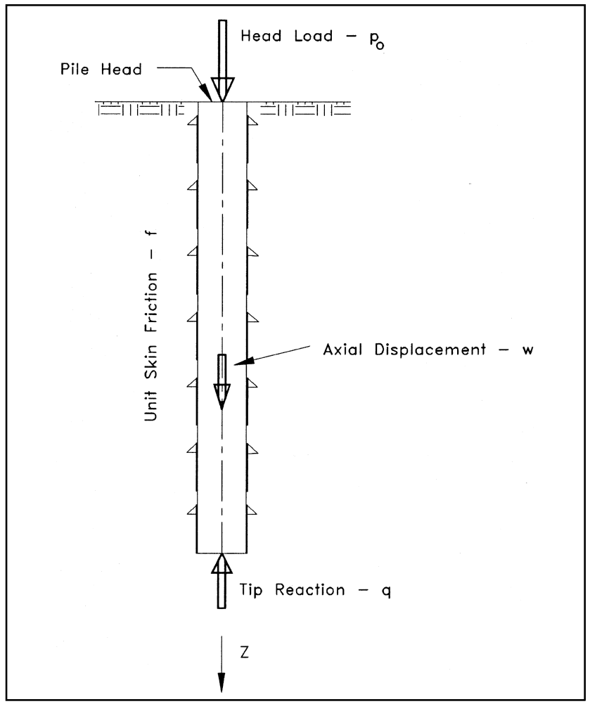
• A necessary prerequisite for a program to be used would be for “typical” t-z curves for various soil types to be developed. The accuracy of the program to predict load-settlement relationships at the pile head depends on the accuracy of the t-z curves at each point along the pile shaft and their counterparts at the pile toe. Determining these was ongoing during the time PX4C3 was being developed, so implementing this was sort of like “building the plane while flying it.” An overview of that topic is given in Mosher and Dawkins’ 2000 work Theoretical Manual for Pile Foundations. (The graphic at the top comes from there.) Much of the work that established Reese as a geotechnical great was his research on the lateral counterparts to t-z curves, the p-y curves, and this effort (in conjunction with the University of Houston’s Mike O’Neill) ran parallel in duration to the t-z curves.
• As noted in his memorial tribute, Lymon Reese founded Ensoft the year after he retired from the University of Texas, which would be 1985. Commercialisation before that would probably run into the university’s conflict of interest policies.

At this point how we got to this point is established. But are we using this technology to the fullest? In the next post we will consider this question.

This is yet another commentary on a paper which cites my work, in this case Inverse analysis for parameter estimation of sandy soil with axially loaded pile using nonlinear programming, which cites Improved Methods for Forward and Inverse Solution of the Wave Equation for Piles. Since 2026 is the tenth anniversary of the publication of that effort, some remarks on why I did that are in order.

Rationale for My Original Study

The current predominant regime in pile dynamics has been around for over half a century now. With tweaks and improvements in computer power and hardware, it has enabled us (well, most of us) to jettison the problematic dynamic formulae for capacity prediction and verification during installation. The whole system, however, relies on the 1D representation of pile/soil interaction to be accurate and the optimization algorithm to find the solution to the inverse problem. Both of these are subject to the kinds of improvements we see in other fields.

Getting to this point was not an easy or straightforward task, both because of the application itself and the code/regulatory environment in which we operate. Much of the struggle to get the current methodology accepted was an uphill battle against the existing “we’ve always done it this way” mentality which settles in, and no doubt this will be the case with a new generation of pile dynamics methodology. But there are some difficult challenges inherent in the physics of this problem, most of which stem from the nature of soils themselves.

I ran into many of these challenges during my study which led to Improved Methods for Forward and Inverse Solution of the Wave Equation for Piles. One colleague from an institution in a neighbouring state felt that my effort was “too ambitious.” He’s probably right, which is why he’s in administration now. But my objective was for this study–and the subsequent papers to fine tune the method–to be a convesation starter, and this paper’s citation of my work is evidence that this is taking place. I sense that efforts to “move the football down the field” in this discipline are taking place, and am gratified to be a part of that effort.

Comments on the Paper Itself

Strictly speaking this paper only has the inverse method as a commonality with my own study. In this case the researchers are dealing with a drilled shaft and are trying to back analyse static capacity. While this sidesteps the rate-dependent problem between dynamic signals and static response, it brings other factors into play, some of which are definite weaknesses in the paper and others where the jury is still out.

Optimisation Technique

Let’s start with one which falls into the latter category: the optimisation technique they chose, which was the Davidon-Fletcher-Powell method. The purpose of optimisation techniques is to find the minima and maxima of “equations” (often they can be expressed in this way, but in this business frequently they can’t) and thus the best solution to the problem. The classic example of this (and one frequently used to test optimisation techniques) is the Rosenbrock Equation, which is

and is plotted as shown below for a =1 and b = 100.

This has challenged optimisation techniques for a long time. The problem with using something aimed at problems like this is that, in geotechnical engineering, problems look less like this and more like relief maps. The result is having to deal with false minima. For example, if we have a canyon on top of a plateau, a false minimum would be the lowest elevation at the bottom of the canyon rather than the bottom of the cliffs of the plateau, which are generally lower. Multiple false minima are common for problems in this profession, which is one reason why we still use brute force grid optimisation in problems like slope stability. This is why I chose a polytope method for my own study, which is derivative free and “casts a wider net” on the downhill slopes of a problem. It is slow and its results not perfect but I think this is a problem that needs to be addressed if we are to use optimisation techniques for solving geotechinical problems.

A couple of side notes:

• I did use a quasi-Newton routine related to the DFP method in my study “Analysis of Vibratory Pile Drivers using Longitudinal and Rotational Oscillations with a Purely Plastic Soil Model” because I felt the parameters were “regular” enough to justify its use. The routine I used had an option for the BFGS (Broyden–Fletcher–Goldfarb–Shanno) method. And that leads to…
• My last course for my PhD degree was in Optimisation. One day our professor–Dr. Kyle Anderson, one of the most brilliant people I’ve come to know–was going on about these techniques, and as you can see Roger Fletcher’s name comes up in many of them. So I leaned over to one of my classmates and said, “Fletcher sure does play both sides of the street.” Dr. Anderson was irritated at seeing whispering, and made me repeat this to the whole class. When I did he thought for a second and said, “He does play both sides of the street.”

The Capacity Issue

In the paper at hand, the optimisation technique starts with initial values and comes to back-analysed values which are then compared to reference values. The problem here is that the reference values are based on single values of toe capacity and soil parameters, the latter of which are related to static methods of analysis. There are two problems which arise in this approach.

The first is the variability of static methods relative to the actual performance of the deep foundation. This is evidenced by the wide scatter in the results these methods return (it’s not quite as bad with drilled shafts as it is with driven piles, but it’s bad enough.)

The second is that the whole business of the “capacity” of deep foundations–ultimate, allowable or factored–cannot be divorced from the fact that the resistance of piles to load takes place through a distance, or settlement. Capacity doesn’t mean much when it’s decoupled from settlement. For static analysis the Holy Grail needs to be that we can estimate the distribution of pile resistance–both between the shaft and the toe and along the shaft–from static load tests. Using static “capacities” may have made the optimisation method they chose possible to use but it does not really get us to where we need to go. Dynamic testing and methods such as CAPWAP recognise this problem but, as noted earlier, improvements there are possible if not easy to arrive at.

Conclusion

I think this paper is an interesting study as a step towards using optimisation techniques to solve the inverse problem of pile resistance to axial load. But there are many more issues to deal with if we are to come to a workable solution for this problem.