
With the basic parameters established, we can turn to the static analysis of the pile, both axial and lateral.
Shaft Resistance Profile
| Depth at Centre of Layer, feet | Soil Shear Modulus, ksf | Beta | Quake,inches | Maximum Load Transfer, ksf | Spring Constant for Wall Shear, ksf/in | Smith-Type Damping Constant, sec/ft | Maximum Load Transfer During Driving (SRD), ksf |
| 0.50 | 48.4 | 0.163 | 0.0022 | 0.009 | 4.03 | 45.394 | 0.009 |
| 1.50 | 83.9 | 0.163 | 0.0038 | 0.027 | 6.99 | 19.911 | 0.027 |
| 2.50 | 108.3 | 0.163 | 0.0050 | 0.045 | 9.02 | 13.572 | 0.045 |
| 3.50 | 128.1 | 0.163 | 0.0059 | 0.063 | 10.68 | 10.543 | 0.063 |
| 4.50 | 145.3 | 0.163 | 0.0067 | 0.081 | 12.11 | 8.730 | 0.081 |
| 5.50 | 160.6 | 0.164 | 0.0074 | 0.098 | 13.38 | 7.509 | 0.098 |
| 6.50 | 174.6 | 0.164 | 0.0080 | 0.116 | 14.55 | 6.623 | 0.116 |
| 7.50 | 187.6 | 0.164 | 0.0086 | 0.134 | 15.63 | 5.948 | 0.134 |
| 8.50 | 199.7 | 0.164 | 0.0091 | 0.152 | 16.64 | 5.414 | 0.152 |
| 9.50 | 211.1 | 0.164 | 0.0097 | 0.170 | 17.59 | 4.980 | 0.170 |
| 10.50 | 222.0 | 0.164 | 0.0102 | 0.188 | 18.50 | 4.618 | 0.188 |
| 11.50 | 232.3 | 0.164 | 0.0106 | 0.206 | 19.36 | 4.313 | 0.206 |
| 12.50 | 242.2 | 0.164 | 0.0111 | 0.224 | 20.18 | 4.050 | 0.224 |
| 13.50 | 251.7 | 0.164 | 0.0115 | 0.242 | 20.98 | 3.822 | 0.242 |
| 14.50 | 260.9 | 0.164 | 0.0120 | 0.260 | 21.74 | 3.621 | 0.260 |
| 15.50 | 269.8 | 0.164 | 0.0124 | 0.278 | 22.48 | 3.444 | 0.278 |
| 16.50 | 278.4 | 0.164 | 0.0128 | 0.296 | 23.20 | 3.285 | 0.296 |
| 17.50 | 286.7 | 0.164 | 0.0132 | 0.314 | 23.89 | 3.142 | 0.314 |
| 18.50 | 294.8 | 0.164 | 0.0135 | 0.332 | 24.57 | 3.013 | 0.332 |
| 19.50 | 302.7 | 0.164 | 0.0139 | 0.351 | 25.22 | 2.895 | 0.351 |
| 20.50 | 310.4 | 0.164 | 0.0143 | 0.369 | 25.86 | 2.787 | 0.369 |
| 21.50 | 317.9 | 0.164 | 0.0146 | 0.387 | 26.49 | 2.688 | 0.387 |
| 22.50 | 325.2 | 0.164 | 0.0149 | 0.405 | 27.10 | 2.597 | 0.405 |
| 23.50 | 332.4 | 0.165 | 0.0153 | 0.423 | 27.70 | 2.512 | 0.423 |
| 24.50 | 339.4 | 0.165 | 0.0156 | 0.441 | 28.29 | 2.434 | 0.441 |
| 25.50 | 346.3 | 0.165 | 0.0159 | 0.460 | 28.86 | 2.361 | 0.460 |
| 26.50 | 353.1 | 0.165 | 0.0162 | 0.478 | 29.42 | 2.292 | 0.478 |
| 27.50 | 359.7 | 0.165 | 0.0166 | 0.496 | 29.98 | 2.228 | 0.496 |
| 28.50 | 366.3 | 0.165 | 0.0169 | 0.515 | 30.52 | 2.168 | 0.515 |
| 29.50 | 372.7 | 0.165 | 0.0172 | 0.533 | 31.06 | 2.112 | 0.533 |
| 30.50 | 379.0 | 0.165 | 0.0175 | 0.552 | 31.58 | 2.058 | 0.552 |
| 31.50 | 385.2 | 0.165 | 0.0178 | 0.570 | 32.10 | 2.007 | 0.570 |
| 32.50 | 391.3 | 0.166 | 0.0181 | 0.589 | 32.61 | 1.960 | 0.589 |
| 33.50 | 397.4 | 0.166 | 0.0183 | 0.607 | 33.11 | 1.914 | 0.607 |
| 34.50 | 403.3 | 0.166 | 0.0186 | 0.626 | 33.61 | 1.871 | 0.626 |
| 35.50 | 409.2 | 0.166 | 0.0189 | 0.645 | 34.10 | 1.830 | 0.645 |
| 36.50 | 415.0 | 0.166 | 0.0192 | 0.664 | 34.58 | 1.790 | 0.664 |
| 37.50 | 420.7 | 0.166 | 0.0195 | 0.683 | 35.06 | 1.753 | 0.683 |
| 38.50 | 426.4 | 0.166 | 0.0197 | 0.702 | 35.53 | 1.717 | 0.702 |
| 39.50 | 432.0 | 0.167 | 0.0200 | 0.721 | 36.00 | 1.682 | 0.721 |
| 40.50 | 437.5 | 0.167 | 0.0203 | 0.740 | 36.46 | 1.649 | 0.740 |
| 41.50 | 443.0 | 0.167 | 0.0206 | 0.759 | 36.92 | 1.618 | 0.759 |
| 42.50 | 448.4 | 0.167 | 0.0208 | 0.778 | 37.37 | 1.587 | 0.778 |
| 43.50 | 453.8 | 0.168 | 0.0211 | 0.798 | 37.82 | 1.558 | 0.798 |
| 44.50 | 459.1 | 0.168 | 0.0214 | 0.817 | 38.26 | 1.530 | 0.817 |
| 45.50 | 464.4 | 0.168 | 0.0216 | 0.837 | 38.70 | 1.502 | 0.837 |
| 46.50 | 469.6 | 0.168 | 0.0219 | 0.856 | 39.13 | 1.476 | 0.856 |
| 47.50 | 474.8 | 0.169 | 0.0221 | 0.876 | 39.56 | 1.450 | 0.876 |
| 48.50 | 479.9 | 0.169 | 0.0224 | 0.896 | 39.99 | 1.426 | 0.896 |
| 49.50 | 485.0 | 0.169 | 0.0227 | 0.916 | 40.42 | 1.402 | 0.916 |
| 50.50 | 489.1 | 0.169 | 0.0229 | 0.933 | 40.76 | 1.382 | 0.933 |
| 51.50 | 492.3 | 0.170 | 0.0231 | 0.947 | 41.03 | 1.367 | 0.947 |
| 52.50 | 495.5 | 0.170 | 0.0233 | 0.960 | 41.30 | 1.352 | 0.960 |
| 53.50 | 498.7 | 0.171 | 0.0234 | 0.974 | 41.56 | 1.337 | 0.974 |
| 54.50 | 501.9 | 0.171 | 0.0236 | 0.988 | 41.83 | 1.323 | 0.988 |
| 55.50 | 505.1 | 0.171 | 0.0238 | 1.002 | 42.09 | 1.308 | 1.002 |
| 56.50 | 508.3 | 0.172 | 0.0240 | 1.016 | 42.36 | 1.294 | 1.016 |
| 57.50 | 511.5 | 0.172 | 0.0242 | 1.031 | 42.63 | 1.280 | 1.031 |
| 58.50 | 514.7 | 0.173 | 0.0244 | 1.045 | 42.89 | 1.266 | 1.045 |
| 59.50 | 517.9 | 0.173 | 0.0246 | 1.060 | 43.16 | 1.252 | 1.060 |
| 60.50 | 521.1 | 0.174 | 0.0248 | 1.075 | 43.42 | 1.238 | 1.075 |
| 61.50 | 524.3 | 0.174 | 0.0250 | 1.091 | 43.69 | 1.224 | 1.091 |
| 62.50 | 527.5 | 0.175 | 0.0252 | 1.106 | 43.96 | 1.211 | 1.106 |
| 63.50 | 530.7 | 0.176 | 0.0254 | 1.122 | 44.22 | 1.197 | 1.122 |
| 64.50 | 533.9 | 0.176 | 0.0256 | 1.139 | 44.49 | 1.184 | 1.139 |
| 65.50 | 537.1 | 0.177 | 0.0258 | 1.155 | 44.76 | 1.170 | 1.155 |
| 66.50 | 540.4 | 0.178 | 0.0260 | 1.172 | 45.03 | 1.157 | 1.172 |
| 67.50 | 543.6 | 0.178 | 0.0262 | 1.189 | 45.30 | 1.144 | 1.189 |
| 68.50 | 546.9 | 0.179 | 0.0265 | 1.207 | 45.57 | 1.130 | 1.207 |
| 69.50 | 550.2 | 0.180 | 0.0267 | 1.224 | 45.85 | 1.117 | 1.224 |
| 70.50 | 553.5 | 0.181 | 0.0269 | 1.243 | 46.12 | 1.104 | 1.243 |
| 71.50 | 556.8 | 0.182 | 0.0272 | 1.262 | 46.40 | 1.091 | 1.262 |
| 72.50 | 560.1 | 0.183 | 0.0274 | 1.281 | 46.68 | 1.078 | 1.281 |
| 73.50 | 563.5 | 0.184 | 0.0277 | 1.300 | 46.96 | 1.065 | 1.300 |
| 74.50 | 566.9 | 0.185 | 0.0280 | 1.321 | 47.24 | 1.051 | 1.321 |
| 75.50 | 570.3 | 0.186 | 0.0282 | 1.341 | 47.52 | 1.038 | 1.341 |
| 76.50 | 573.7 | 0.187 | 0.0285 | 1.363 | 47.81 | 1.025 | 1.363 |
| 77.50 | 577.2 | 0.188 | 0.0288 | 1.385 | 48.10 | 1.012 | 1.385 |
| 78.50 | 580.7 | 0.190 | 0.0291 | 1.407 | 48.39 | 0.999 | 1.407 |
| 79.50 | 584.3 | 0.191 | 0.0294 | 1.431 | 48.69 | 0.985 | 1.431 |
| 80.50 | 587.9 | 0.193 | 0.0297 | 1.455 | 48.99 | 0.972 | 1.455 |
| 81.50 | 591.5 | 0.194 | 0.0300 | 1.479 | 49.29 | 0.959 | 1.479 |
| 82.50 | 595.2 | 0.196 | 0.0303 | 1.505 | 49.60 | 0.945 | 1.505 |
| 83.50 | 598.9 | 0.197 | 0.0307 | 1.532 | 49.91 | 0.932 | 1.532 |
| 84.50 | 602.7 | 0.199 | 0.0310 | 1.559 | 50.22 | 0.919 | 1.559 |
| 85.50 | 606.5 | 0.201 | 0.0314 | 1.587 | 50.54 | 0.905 | 1.587 |
| 86.50 | 610.4 | 0.203 | 0.0318 | 1.617 | 50.87 | 0.891 | 1.617 |
| 87.50 | 614.4 | 0.205 | 0.0322 | 1.647 | 51.20 | 0.878 | 1.647 |
| 88.50 | 618.4 | 0.207 | 0.0326 | 1.678 | 51.53 | 0.864 | 1.678 |
| 89.50 | 622.5 | 0.210 | 0.0330 | 1.711 | 51.87 | 0.850 | 1.711 |
| 90.50 | 626.7 | 0.212 | 0.0334 | 1.745 | 52.22 | 0.837 | 1.745 |
| 91.50 | 630.9 | 0.215 | 0.0339 | 1.781 | 52.58 | 0.823 | 1.781 |
| 92.50 | 635.2 | 0.217 | 0.0343 | 1.817 | 52.94 | 0.809 | 1.817 |
| 93.50 | 639.7 | 0.220 | 0.0348 | 1.856 | 53.30 | 0.795 | 1.856 |
| 94.50 | 644.2 | 0.223 | 0.0353 | 1.896 | 53.68 | 0.781 | 1.896 |
| 95.50 | 648.8 | 0.226 | 0.0358 | 1.937 | 54.07 | 0.767 | 1.937 |
| 96.50 | 653.5 | 0.229 | 0.0364 | 1.981 | 54.46 | 0.753 | 1.981 |
| 97.50 | 658.3 | 0.233 | 0.0369 | 2.026 | 54.86 | 0.739 | 2.026 |
| 98.50 | 663.3 | 0.236 | 0.0375 | 2.073 | 55.27 | 0.725 | 2.073 |
| 99.50 | 668.3 | 0.240 | 0.0381 | 2.122 | 55.69 | 0.710 | 2.122 |
The results should be self explanatory; however, some observations are in order.
- A 1′ increment was used for the analysis. This will be carried over to both the static and dynamic axial analyses. For this routine it’s probably overkill, but for a real system with multiple soil layers this eliminates a great deal of interpolation and adjustment.
- Both the shear modulus and the maximum shear stress on the shaft surface vary with effective stress. This tends to homogenise the quake to some degree. The increase of shear modulus with depth also increases the shaft element stiffness as well.
- Beta values are about 50% higher at the pile toe than at the pile head. This is mostly due to the depth effect of the
value computed by the method used.
- The resulting quakes are lower than the “traditional values.” This varies from run to run.
- The Smith-type damping constants are considerably higher than is usually expected. This will be discussed with the wave equation analysis itself.
- There is no difference between ultimate capacity and SRD with this run because of the cohesionless soils. This will change with cohesive ones.
ALP Program
The original routine used the PX4C3 routine to construct the axial load-deflection curve. For this routine it was replaced by the ALP program, which is described in Verruijt. The Turbo Pascal code in the text was converted to php and modified for the online application. The ALP99 program, which allows for layered soils, has been used in a classroom setting, is a good program but has three serious weaknesses:
- There is no guidance on what values of quake to use for either shaft or toe, and for beginners this is very confusing.
- The guidance on entering shaft resistance properties is primitive, to say the least.
- The program simply crashes if a resistance in excess of the ultimate resistance is entered, even though the latter is easily computed.
This online version of ALP addresses all of these by limiting the highest resistance during the “load test” and furnishing quake and resistance values all along the shaft and toe.
The basic parameters of ALP returned by TAMWAVE are shown below.
| Length of the pile, in. | 1,200.0 |
| Axial stiffness EA. lbs. | 720,000,000 |
| Circumference, in. | 48.000 |
| Point resistance, lbs. | 202,673 |
| Quake of the point, in. | 0.879 |
| Number of pile elements | 100 |
| Number of loading steps | 20 |
| Maximum pile load, lbs. | 572,676.9 |
| Load Increment, lbs. | 57,267.7 |
| Failure Load, lbs. | 572,676.9 |
Some of these are repetitious from earlier data output. The results of the actual “load test” are shown below.
| Load Step | Force at Pile Head, kips | Pile Head Deflection, in. | Number of Plastic Shaft Springs |
| 0 | 0.0 | 0.000 | 0 |
| 1 | 57.3 | 0.033 | 22 |
| 2 | 114.5 | 0.082 | 39 |
| 3 | 171.8 | 0.144 | 52 |
| 4 | 229.1 | 0.216 | 64 |
| 5 | 286.3 | 0.300 | 74 |
| 6 | 343.6 | 0.395 | 85 |
| 7 | 400.9 | 0.601 | 100 |
| 8 | 343.6 | 0.571 | 10 |
| 9 | 286.3 | 0.534 | 22 |
| 10 | 229.1 | 0.489 | 31 |
| 11 | 171.8 | 0.437 | 39 |
| 12 | 114.5 | 0.378 | 45 |
| 13 | 57.3 | 0.314 | 52 |
| 14 | 0.0 | 0.244 | 58 |
The program ceases to load the pile and begins to unload when all of the shaft friction is mobilised or the ultimate load is achieved, whichever comes first. This is intended to prevent the routine from going unstable with the applied load too near the maximum capacity of the pile, thus violating static equilibrium.
ALP solves the system by constructing a tridiagonal matrix and then solving the non-linear problem. In some cases it will achieve a result before coming to actual convergence according to the convergence criterion. In such cases ALP will report that no convergence was achieved.

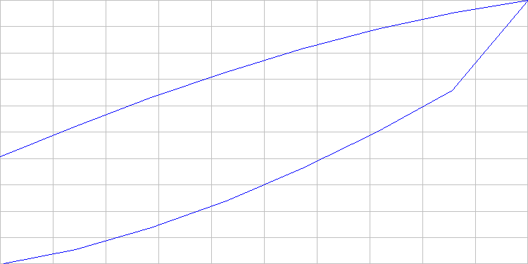
x-axis = Pile Head Force
y-axis = Pile Head Deflection
Plot Limits:
x-axis from 0.000 to 400.874
y-axis from 0.000 to 0.601
One new feature with the current version of TAMWAVE is the inclusion of two basic graphs of the results. This is one of them. Contrary to American practice, the deflection (y) axis is upward even though the actual deflection is downward. For serious plotting purposes it is probably best for the student to copy and paste the results into a spreadsheet or other plotting program and then make the results look more presentable.
CLM 2 Routine for Lateral Loads
To analyse lateral pile loading, the CLM2 Method is employed. Details on this method can be found with the CLM 2 spreadsheet here. Some notes about this are as follows:
- The analyser is for single piles only, no group or bent analysis.
- The following cases can be considered:
- Free (Pinned) Head, Lateral Force Only
- Free Head, Moment Only
- Free Head, Combined Force and Moment
- Fixed Head, Lateral Force Only
- Any lateral load or pile head moment is entered when the soil properties are confirmed. If zero load or moment is entered, the results are expanded or truncated accordingly.
For this example the results of the CLM 2 analysis are here.
| Nominal Soil Unit Weight, lb/in3 | 0.06944 |
| Pile Moment of Inertia, in4 | 1,728.00 |
| Pile Section Modulus, in3 | 288.00 |
| Pile Solid Circle Moment of Inertia, in4 | 1,017.88 |
| Moment of Inertia Ratio Ri | 1.698 |
| Pile Moment of Inertia Ratio Product, ksi | 8,488.3 |
| Pile-Soil Interaction Variable | 97,803 |
| Pile L/D Ratio | 100.0 |
| Characteristic Load, lbs. | 2,745,232.8 |
| Characteristic Moment, in-lbs. | 196,821,533.6 |
| Pile Head Fixity | Free |
| Pile Head Lateral Load, lbs. | 5,000.0 |
| Pt/Pc | 0.00182 |
| Yt/D | 0.00800 |
| Pile Head Deflection due to Load, inches | 0.096 |
| Maximum Moment Due to Pile Head Lateral Load, in-lbs | 136,112.3 |
| Maximum Bending Stress Due to Pile Head Lateral Load, in-lbs | 472.6 |
The results are explained in the CLM 2 documentation. The bending stresses are not really meaningful in concrete piles, as flexure is generally transmitted through the reinforcement. Parametric studies must be run manually, i.e., one load at a time.
CLM 2 is a quick way to obtain estimates of lateral loads, shears and moments for groundline piles and simple soil profiles, and both of these are present in TAMWAVE. Since all of the soil input is already done, this source of error is eliminated.
Once these results are complete, the user can proceed to run a wave equation analysis.

Reblogged this on vulcanhammer.info.
LikeLike