
Although the need for many of the tables is a thing of the past, this is still a useful reference for mathematical functions such as integral tables, physical constants and Laplace transforms. It also includes the elliptic integrals which find use with the Boussinesq equations for circular loads on elastic media.
Category: Academic Issues
Explaining the Relationship Between the Coefficient and the Angle of Friction
One of the things that gets covered (if not very thoroughly) in Soil Mechanics is how friction is developed in soils. An analogy is made with the classic “block on a surface” problem we see in Statics, but the tie-in isn’t as strong as one would like.
The fact is that, for purely cohesionless soils, the friction between the particles and the friction between the surface and the block is basically the same Coulombic friction. As is usually the case in soil mechanics, how that actually plays out in soil properties has many complexities, but then again surface friction isn’t a simple or straightforward property in and of itself.
Another part of the problem is that, in Statics, friction isn’t taught with geotechnical considerations in mind, especially these days. This is a pity, not only for those of us in the geotechnical community but for those who work with granular materials on a production or use basis.
This is a brief treatment of the subject, basing the development of the topic from that in Movnin and Izrayelit (1970), which comes closer to relating the two quantities we see to define friction: the friction angle and the friction coefficient.
The Basics of the Friction Coefficient and Angle

Surface friction comes from the rubbing of two surfaces together, as shown at the right. We see the three forces with which the two surfaces interact: the normal force N, the resulting friction force F and the resultant of the two R. We also see that the addition of lubricant is important in that it separates the two surfaces and reduces the effect of the asperities on each other, something that contractor and engineer alike frequently overlook in both the maintenance and performance evaluation of the equipment.
The normal and frictional forces resisting the relative motion of the two surfaces is related by the equation
F = fN (1)
With granular materials, the main difference is that the surfaces of the particles aren’t straight at all but they do rub up against each other, the asperities on the particle surface contributing to the mutual resistance of the particles. Although water acts to a limited extent as a lubricant, its largest effect is the buoyant effect on the intergranular (effective) stress, as shown below.

Returning to the first diagram, without any mutual pressure of the surfaces (the normal force N) there is no friction force F tangential to the surface. Again in soil mechanics purely cohesionless (granular) soils have no frictional strength unless weight or other pressure is applied to them.

Now let us consider the diagram at the right. The normal force N exerted by the surface on the block (caused by the force exerted on the block Q) and the frictional force F (caused by the force P which attempts to move the block) add vectorially to a resultant R, which in turn has an angle with the normal force N. The geometry of the forces and Equation (1) relate the angle to the friction factor as
f = F/N = tan (φ) (2)
Cone of Friction
Although F and N are related through both Equations (1) and (2), in reality F cannot exist without some tangential force pushing the block. This is the force P which is attempting to push the block along the plane. As P increases F increases until we get to a point where we have impending motion, beyond which the block moves and begins to accelerate. The value of f or φ when impending motion turns into actual motion is when we reach the ultimate value of f or φ, which we will designate as f0 or φ0.
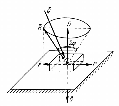
These form a “cone of friction.” This cone of friction can be seen in the diagram at the left. As long as F < f0 N (or F < tan (φ0) N) and the resultant Q of N and F is within the cone, the block is motionless. Beyond that point it moves, and the coefficient of friction in motion can be different (usually smaller) than the coefficient of friction at the point of impending motion.
It is here that we can relate the friction factor f and the angle of friction φ can be related to each other and to concepts familiar to geotechnical people. When we construct the Mohr-Coulomb diagram, we define a failure envelope of legal stress states (within the envelope) and illegal stress states (outside the envelope.) We can see all of these with the failure function below. When the failure function is negative (1), we are within the envelope and failure does not take place. When the failure function is zero (2), we have impending failure. When the failure function is positive (3), we have failure and an illegal stress state.

Three-dimensional envelopes are certainly common in geotechnics, especially in finite elements. An example of this is shown below.

Determining the Friction Factor or Angle

To determine the friction angle, one simple way is to start with a block and a level surface and then raise the angle of the surface until the block moves. Such an apparatus is shown at the left.
As the angle α increases the direction of the weight G relative to the surface changes in can be divided into two parts: the normal force G2 and the tangential force G1. The latter will move the block down but it is resisted by the friction force F, which will resist until G1 > F0, at which point the block will start to move down the slope at a constant acceleration. By noting the angle at which this takes place, both f0 or φ0 = α0 can be determined. The math for this is similar to the level surface and block.
The geotechnical counterpart to this is the angle of repose. Suppose we allow a small stream of sand to drop on a surface. Over time the sand will build up into a conical pile with the surface at an angle to the flat surface the sand is streamed onto. This angle is referred to as the angle of repose. In theory the angle of repose is equal to the friction angle of the soil, although with the usual complexities of geotechnics this isn’t always the case. There are clean sands with which we can use the angle of repose to estimate the internal friction angle of the soil. When I was teaching at UTC, some of the students were working on the ASCE MSE Wall project and needed a friction value for the sand being used in the box. While they were looking at direct shear or triaxial testing, I suggested using the angle of repose to get a “ballpark” value. They did this and it was helpful.
Some Comments
- The use of the angle of friction has fallen out of favour in engineering education, which is one reason why it is difficult to relate friction as taught in Statics to friction as used in geotechnical engineering. That wasn’t always the case; one example from the early twentieth century is Tapered Keys and Their Use In Vulcan Hammers.
- Hopefully this treatment of the subject will be useful to students to help them relate the concept of friction in statics to that in geotechnical engineering.
RIP Lee L. Lowery, Jr.
Driven Pile Design Series Now Available
Of all the topics I taught in my course on foundation design and analysis, my favourite topic was driven piles. I have taken this part of the course and am presenting it on the companion site vulcanhammer.info. The topics are as follows:
- Driven Pile Design: Introduction and Overview
- Driven Pile Design: Axial Loads, General Considerations
- Driven Pile Design: Three Methods of Analysis
- Driven Pile Design: Static Load Testing and Axial Settlement
- Driven Pile Design: Axial Group Bearing Capacity and Settlement
- Driven Pile Design: Lateral Loads on Piles
- Driven Pile Design: Wave Equation Analysis
- Driven Pile Design: Inverse and Verification Methods
- Driven Pile Design: ASD and LRFD Methods
In putting this together, I added some material, including a different example problem and actual runs of axial and lateral load software, along with the wave equation analysis.
I trust that you will find this enjoyable and profitable.
Closing the Loop (or at least trying to) on Hough’s Settlement Method
My post Getting to the Legacy of B.K. Hough and his Settlement Method got a good amount of interest. Unfortunately it left several “loose ends,” some of which is because we don’t have full information on some of Hough’s methodology, and others because we don’t have full information on the FHWA’s thinking in their resurrection of the method. The objective of this post is to clear up some of these loose ends, especially the latter.
What we needed was some additional information on the background for both Hough’s work and the FHWA’s interpretation of that work. That information came from an unexpected source: the FHWA’s Design and Construction of Driven Pile Foundations, 2016 Edition. This has been available on vulcanhammer.info just about since it was first published. Now some of you are asking, “Why is this guy waiting until now to come out with stuff he’s had for years? Doesn’t he read the material he offers for download?” In my defence, I didn’t expect the solution to come from the driven pile manual, since it’s primarily a shallow foundation issue. It’s there because it’s proposed for use with groups of driven piles in cohesionless soils.
With all that said let’s look at some of the issues this “new” source tackles.
The SPT Correction Issue
The basic equation for Hough’s method is similar to that used for one-dimensional consolidation settlement and is

where
settlement of cohesionless soil layer
layer thickness
compression coefficient
effective stress at the centre of the layer
effective stress at the centre of the layer plus the induced stress from the surface at the centre of the layer
The tricky part has always been 
- Hough’s Method may or may not have used a 60% (N60) efficient hammer to develop the method. It’s entirely possible but Hough (1959) doesn’t say what type of hammer he used to develop the method.
- The FHWA implementation of Hough’s method included an SPT correction for overburden, which was absent in Hough (1959.)
- An absence of any mention of Hough (1969,) where he modified the
values.
- The lack of an attempt to convert the chart to equations. My original post demonstrates how this can be done, using the method of Hough (1969.)
Design and Construction of Driven Pile Foundations, 2016 Edition addresses all of this as follows:
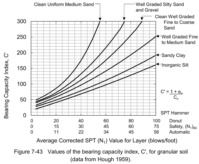
Cheney and Chassie (2002) report that FHWA experience with this method indicates the method is usually conservative and can overestimate settlements by a factor of 2. This conservatism is attributed to the use of the original bearing capacity index chart from Hough (1959) which was based upon SPT donut hammer data. Based upon average energy variations between SPT donut, safety, and automatic hammers reported in technical literature, Figure 7-43 now includes a correlation between SPT N values from safety and automatic hammers and bearing capacity index. The safety hammer values are considered N60 values. This modification should improve the accuracy of settlement estimates with this method.
The following should be noted about these changes:
- The assumption that Hough used a “donut” hammer is a reasonable one based on the technology of the time, but it’s still an assumption. Hough doesn’t tell us the kind of SPT hammer he used, or even how he came up with the C’ values shown above.
- The chart above (Figure 7-43) shows the correlation for three types of hammers: donut, safety, and automatic hammers (which now “rule the roost” in testing.) However, it still insist that the safety hammer values should be corrected for overburden, something else absent from Hough’s study.
- There is still no awareness of Hough (1969.)
So we can say that we have, perhaps, made some progress toward a solution, but at this point we are not quite where we would like to be.
My Thinking on the Way Forward
We usually think in terms of progress in this field in terms of peer-reviewed articles. But we’ve had the peer-reviewed articles, the experts weigh in on what they mean, and another set of experts try to make things better. My own solution to this problem would run like this:
- Let’s accept the FHWA’s idea that Hough used a donut hammer for his original work. Donut hammers have a “standard” efficiency of 45%. To get the SPT blow counts to an N60 value (60% efficiency) we need to divide the donut SPT values by 60/45 = 4/3. (That’s what’s going on in the graph above.)
- Let’s use Hough’s method as he presented it in Hough (1969) and assume that those values too came from donut hammers.
- Let’s lose the overburden correction; it wasn’t in the original and I don’t see how one can justify putting it into this method.
If we implement all of this, the chart now looks like this:
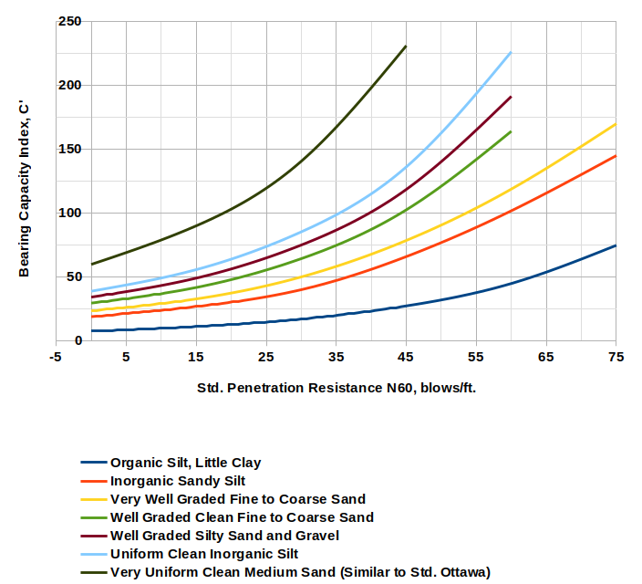
If formulae are preferred (and that’s normally the case these days) they will again be in the form

and the coefficients will be as follows:
| Soil Type | A | B |
| Organic Silt, Little Clay | 7.22 | 0.0305 |
| Inorganic Sandy Silt | 18.27 | 0.0279 |
| Very Well Graded Fine to Coarse Sand | 22.86 | 0.0270 |
| Well Graded Clean Fine to Coarse Sand | 28.22 | 0.0289 |
| Well Graded Silty Sand and Gravel | 32.85 | 0.0289 |
| Uniform Clean Inorganic Silt | 37.02 | 0.0294 |
| Very Uniform Clean Medium Sand (Similar to Std. Ottawa) | 58.66 | 0.0299 |
The “B” coefficients run in a fairly narrow range and have an average of 0.0289. It’s possible using this or a more sophisticated method to apply the same value of B to all of the soils.
Any comments from those of you who have used Hough’s Method, or have research on the topic, would be greatly appreciated.
References
- Hough, B.K. (1959). “Compressibilty as the Basis for Soil Bearing Value,” Journal of the Soil Mechanics and Foundations Division, ASCE, Vol. 85, Part 2.
- Hough, B.K. (1969). Basic Soils Engineering. Second Edition. New York: Ronald Press Company.
