Academic Issues – Page 3 – vulcanhammer.net

Closing the Loop (or at least trying to) on Hough’s Settlement Method

Posted on 4 June 202413 June 2025 by Don Warrington

My post Getting to the Legacy of B.K. Hough and his Settlement Method got a good amount of interest. Unfortunately it left several “loose ends,” some of which is because we don’t have full information on some of Hough’s methodology, and others because we don’t have full information on the FHWA’s thinking in their resurrection of the method. The objective of this post is to clear up some of these loose ends, especially the latter.

What we needed was some additional information on the background for both Hough’s work and the FHWA’s interpretation of that work. That information came from an unexpected source: the FHWA’s Design and Construction of Driven Pile Foundations, 2016 Edition. This has been available on vulcanhammer.info just about since it was first published. Now some of you are asking, “Why is this guy waiting until now to come out with stuff he’s had for years? Doesn’t he read the material he offers for download?” In my defence, I didn’t expect the solution to come from the driven pile manual, since it’s primarily a shallow foundation issue. It’s there because it’s proposed for use with groups of driven piles in cohesionless soils.

With all that said let’s look at some of the issues this “new” source tackles.

The SPT Correction Issue

The basic equation for Hough’s method is similar to that used for one-dimensional consolidation settlement and is

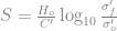
$S=\frac{H_{o}}{C'} \log_{10} \frac{\sigma'_f}{\sigma'_o}$ (1)

where

$S =$ settlement of cohesionless soil layer
$H_o =$ layer thickness
$C' =$ compression coefficient
$\sigma'_o =$ effective stress at the centre of the layer
$\sigma'_f =$ effective stress at the centre of the layer plus the induced stress from the surface at the centre of the layer

The tricky part has always been $C'$ . My criticisms of the FHWA’s implementation of the method in the post Getting to the Legacy of B.K. Hough and his Settlement Method were as follows:

Hough’s Method may or may not have used a 60% (N₆₀) efficient hammer to develop the method. It’s entirely possible but Hough (1959) doesn’t say what type of hammer he used to develop the method.
The FHWA implementation of Hough’s method included an SPT correction for overburden, which was absent in Hough (1959.)
An absence of any mention of Hough (1969,) where he modified the $C'$ values.
The lack of an attempt to convert the chart to equations. My original post demonstrates how this can be done, using the method of Hough (1969.)

Design and Construction of Driven Pile Foundations, 2016 Edition addresses all of this as follows:

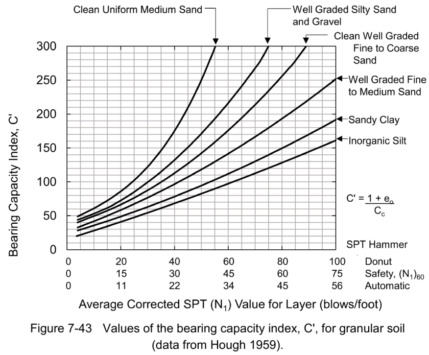
Cheney and Chassie (2002) report that FHWA experience with this method indicates the method is usually conservative and can overestimate settlements by a factor of 2. This conservatism is attributed to the use of the original bearing capacity index chart from Hough (1959) which was based upon SPT donut hammer data. Based upon average energy variations between SPT donut, safety, and automatic hammers reported in technical literature, Figure 7-43 now includes a correlation between SPT N values from safety and automatic hammers and bearing capacity index. The safety hammer values are considered N60 values. This modification should improve the accuracy of settlement estimates with this method.

The following should be noted about these changes:

The assumption that Hough used a “donut” hammer is a reasonable one based on the technology of the time, but it’s still an assumption. Hough doesn’t tell us the kind of SPT hammer he used, or even how he came up with the C’ values shown above.
The chart above (Figure 7-43) shows the correlation for three types of hammers: donut, safety, and automatic hammers (which now “rule the roost” in testing.) However, it still insist that the safety hammer values should be corrected for overburden, something else absent from Hough’s study.
There is still no awareness of Hough (1969.)

So we can say that we have, perhaps, made some progress toward a solution, but at this point we are not quite where we would like to be.

My Thinking on the Way Forward

We usually think in terms of progress in this field in terms of peer-reviewed articles. But we’ve had the peer-reviewed articles, the experts weigh in on what they mean, and another set of experts try to make things better. My own solution to this problem would run like this:

Let’s accept the FHWA’s idea that Hough used a donut hammer for his original work. Donut hammers have a “standard” efficiency of 45%. To get the SPT blow counts to an N₆₀ value (60% efficiency) we need to divide the donut SPT values by 60/45 = 4/3. (That’s what’s going on in the graph above.)
Let’s use Hough’s method as he presented it in Hough (1969) and assume that those values too came from donut hammers.
Let’s lose the overburden correction; it wasn’t in the original and I don’t see how one can justify putting it into this method.

If we implement all of this, the chart now looks like this:

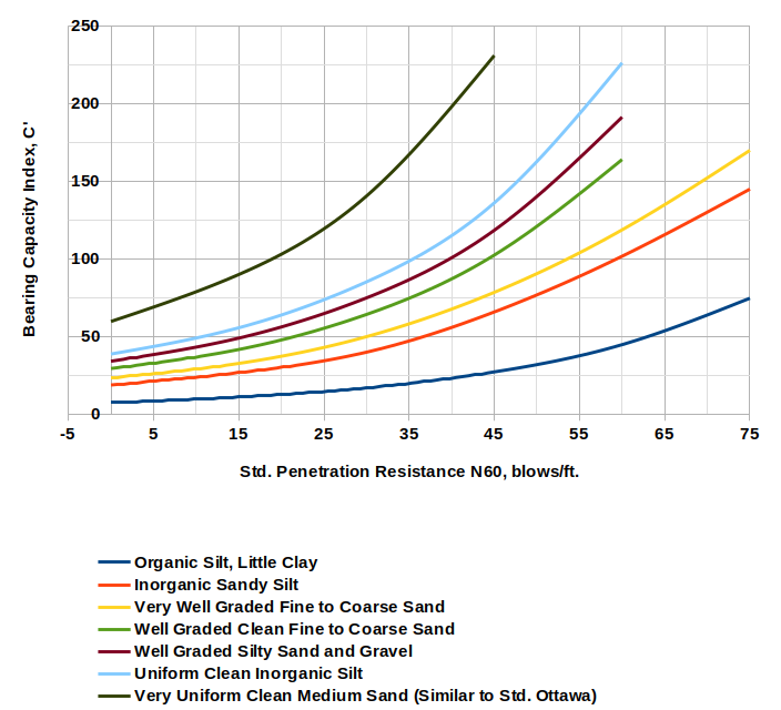
If formulae are preferred (and that’s normally the case these days) they will again be in the form

$C' = A \exp^{BN}$ (2)

and the coefficients will be as follows:

Soil Type	A	B
Organic Silt, Little Clay	7.22	0.0305
Inorganic Sandy Silt	18.27	0.0279
Very Well Graded Fine to Coarse Sand	22.86	0.0270
Well Graded Clean Fine to Coarse Sand	28.22	0.0289
Well Graded Silty Sand and Gravel	32.85	0.0289
Uniform Clean Inorganic Silt	37.02	0.0294
Very Uniform Clean Medium Sand (Similar to Std. Ottawa)	58.66	0.0299

The “B” coefficients run in a fairly narrow range and have an average of 0.0289. It’s possible using this or a more sophisticated method to apply the same value of B to all of the soils.

Any comments from those of you who have used Hough’s Method, or have research on the topic, would be greatly appreciated.

References

Hough, B.K. (1959). “Compressibilty as the Basis for Soil Bearing Value,” Journal of the Soil Mechanics and Foundations Division, ASCE, Vol. 85, Part 2.
Hough, B.K. (1969). Basic Soils Engineering. Second Edition. New York: Ronald Press Company.

Seepage and Bottom Heave Calculations for Sheet Pile Braced Cut Trenches

Posted on 9 May 2024 by Don Warrington

Part of Soils in Construction‘s presentation of dewatering is this topic. I cover it in my treatment of flow nets in Soil Mechanics: Groundwater and Permeability II; however, Soils in Construction uses a less computationally intensive approach. In this piece I’ll explain that, give some better graphics than the book had available at the time of publication, and compare them with the flow net/FEA results I discussed in my Soil Mechanics course.

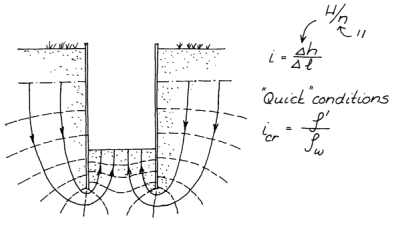
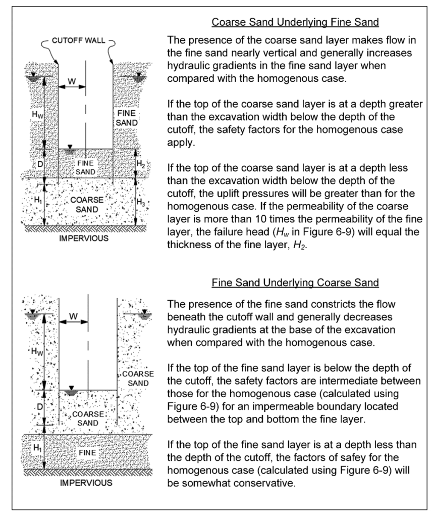
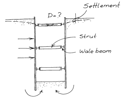
Let us consider the problem of a braced cut, which is commonly used for “cut and cover” construction. Such a construction is shown at the right. One of the challenges of temporary works such as this is to insure that a) there is sufficient pumping capacity to keep the “steel trench” dry, and b) the hydraulic gradient of the water coming up into the trench is sufficiently low to avoid soil boiling and bottom heave due to that soil boiling. (Bottom heave can take place due to other factors as well.) An example of that (showing a flow net) is below to the left.

Because the cut is internally braced, it is usually possible to make the sheeting walls simply penetrate to just below the bottom of the trench. However, in order to mitigate the effects of water flowing from around the cut into the bottom, the sheeting can be extended. The idea is that, the longer the extensions, the longer distance the water has to flow, the increased resistance of the soil to flow, and the lower the hydraulic gradients, which both reduce the flow overall and the possibility that the soil at the bottom of the trench will boil, i.e., enter into a quick condition.

Soils in Construction shows two methods of dealing with this problem:

A “rule of thumb” for sheeting extension; and
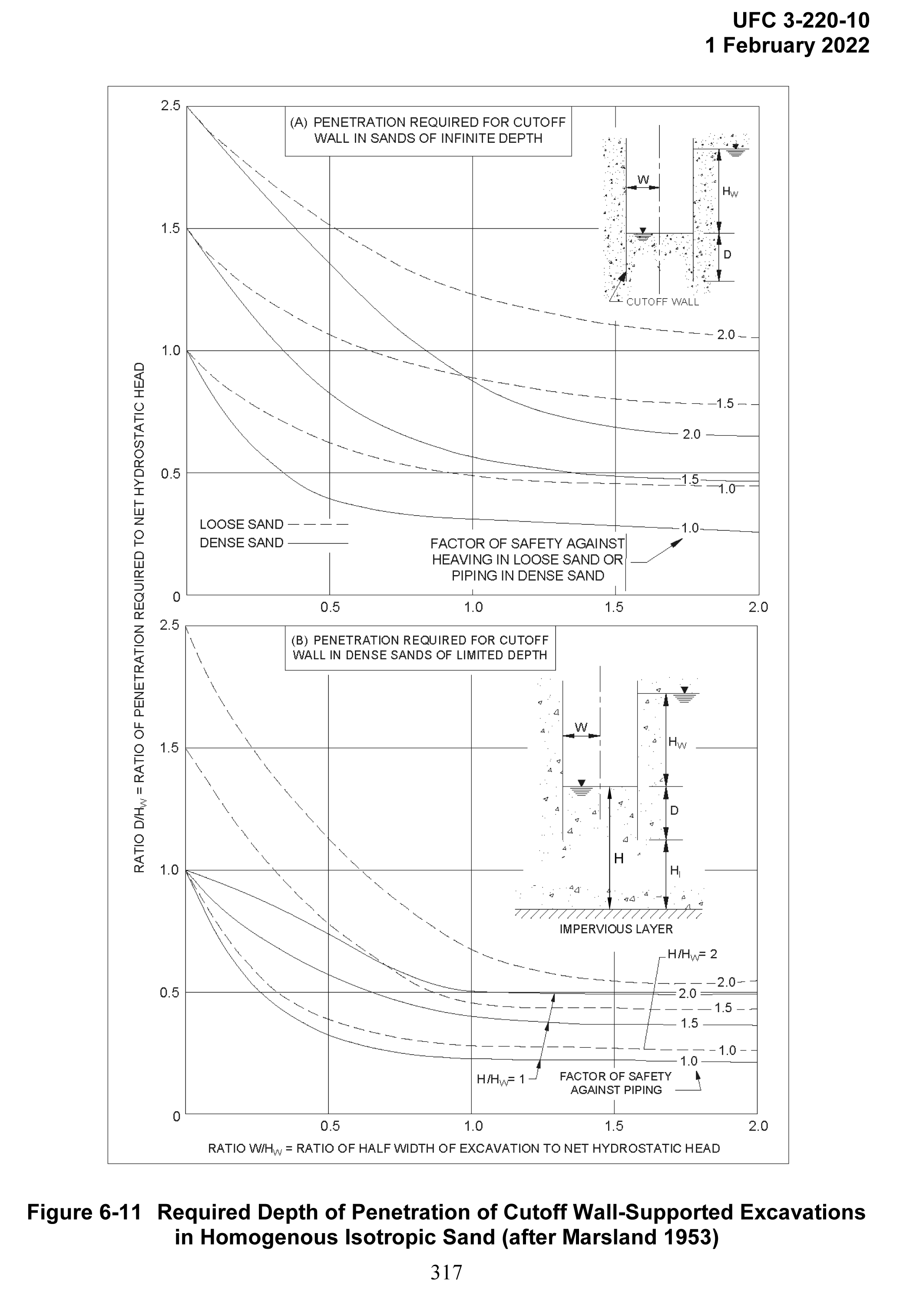
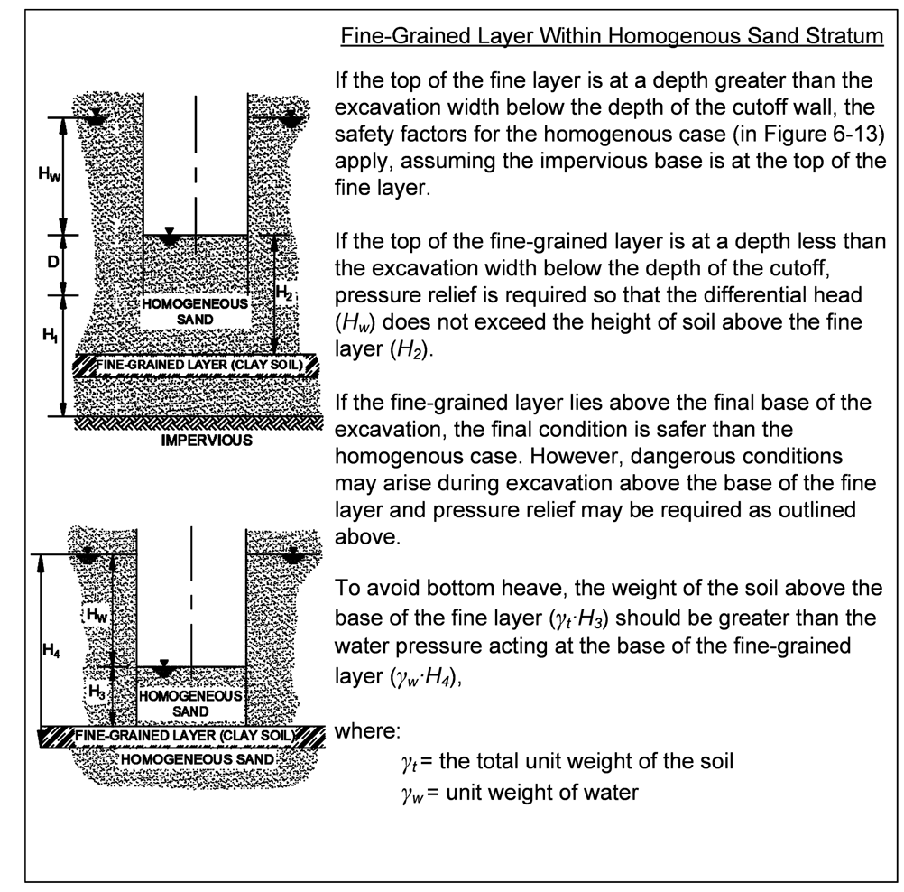
Charts to determine the minimum extension of the sheeting. These were developed by Marsland (1953). In the book they were taken from NAVFAC DM 7.01, but since the book’s publication NAVFAC DM 7.1 has redone the graphics, and you can see that below (and click on it to download). It is important to note that there is an error in the lower part of this figure; I checked it against Marsland (1953) and have modified it a bit to restore it to Marsland’s original formulation, the following example will show how it is supposed to be used.

Example Problem

I have used this example for many years and feature it in Soil Mechanics: Groundwater and Permeability II. Consider the braced cut shown below.

The parameters for this problem are as follows:

Braced Sheet Piling Excavation
- Depth of excavation = 38’
- Width of excavation = 32’
- Impervious layer 20’ below the toe of the sheeting
- Length of Sheet Piling = 66’
Water table at the excavation level on the excavation side
Water table 6’ below the top of the sheeting on the soil side
Variables for chart above
- H_w = 38 – 6 = 32′
- D = 66 – 38 = 28′
- H_l= 20′
- H = D + H_l = 28 + 20 = 48′
- W = 16′
- Even though the graphic for the problem doesn’t show it, the problem statement indicates an impervious layer below the excavation; thus, we will use the lower chart for this problem.
Soil Conditions
- Uniform medium sand, k = 0.0003 ft/sec
- Saturated Unit Weight = 115 pcf

We need to, one way or another, insure that the design does not experience soil boiling.

The “rule of thumb” in Soils in Construction states that “the depth of penetration of the cut-off wall below the bottom of the excavation should be a third of the “length” computed. For this wall, the ratio is 28/66 = 42%, which means the rule of thumb is achieved.

Turning to the chart above, we must compute three quantities:

The x-axis ratio of half width of excavation to net hydrostatic head, or W/H_w = 16/32 = 0.5;
the y-axis ratio of penetration required to net hydrostatic head, or D/H_w = 28/32 = 0.875; and
the ratio of the depth between the bottom of the excavation and the impervious layer to the net hydrostatic head, or H/H_w = 48/32 = 1.5.

In this case we only have two values of H/H_w to work with: 1 and 2. For H/H_w = 1, FS ~ 2.5 (this is a very rough extrapolation.) For H/H_w = 2, FS = 1.75. Since H/H_w = 1.5 is in the middle between the two, the FS = (2.5+1.75)/2 = 2.125.

If we want to check our results by neglecting the impervious layer, we use the upper chart, and assuming the soil is closer to being a loose sand, FS ~ 1.4.

So how does this all compare to a flow net/FEA result? Same is given below.

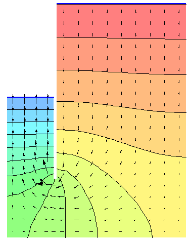
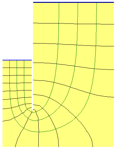
At the right is a flow net generated by the finite element program SEEP-W. At the left is a chart showing the direction of the water flow (arrows) and the hydraulic head (coloured bands.) An in-depth explanation of these can be found at Soil Mechanics: Groundwater and Permeability II. The results are as follows:

Gradient at bottom of excavation = 0.48
Factor of safety = 1.77
Total flow = 1.02 gpm/ft of wall

The critical hydraulic gradient, computed by the methods shown in Computing Pore Water Pressure and Effective Stress in Upward (and Downward) Flow in Soil, is 115/62.4 – 1 = 0.843, which checks with the factor of safety for the actual gradient.

The factor of safety from the chart ignoring the presence of the impervious layer is the closest to the FEA/flow net result. For the chart with the impervious layer, the extrapolation for the lower factor of safety should perhaps be ignored.

A couple of other charts (based on Marsland (1953)) are shown below.

References

Marsland, A.R. 1953. “Model Experiments to Study the Influence of Seepage on the Stability of a Sheeted Excavation in Sand.” Geotechnique, 3(6), 223-241.

Academic Issues, Geotechnical Engineering

The 2:1 Method for Estimating Stresses Under Foundations

Posted on 29 April 202416 June 2025 by Don Warrington

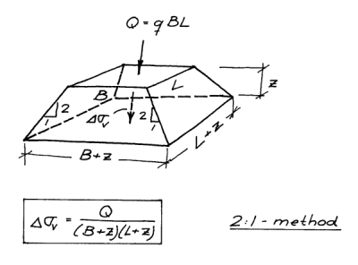
Readers of my post Analytical Boussinesq Solutions for Strip, Square and Rectangular Loads and those related to it know that the math related to these methods can get complicated, and in any case the idea of a “purely elastic” soil response to load is purely theoretical. So is there a simpler way? The most common simplification used is the 2:1 Method, shown at the right.

The method basically assumes the following:

Uniformly loaded foundation
Only stresses of interest are under the centroid of the foundation, as shown, and only vertical stresses are considered
Stresses decrease as if there is a truncated pyramid below the foundation with a slope of 1H:2V.

As shown, to determine the additional vertical stress $\Delta \sigma_v$ at a distance $z$ below the centre of the foundation, the equation for a rectangular foundation of width B and length L (can be interchanged, but conventionally B is the smaller of the two) for a load Q on the surface is given by the equation

$\Delta \sigma_v = \frac{Q}{(B+z)(L+Z)}$ (1)

If the equation is written in terms of the unit load q, it becomes

$\Delta \sigma_v = \frac{q}{(1+\frac{z}{B})(1+\frac{z}{L})}$ (2)

Obviously for square foundations $B=L$ but the solution is the same.

Formulating the problem as shown in Equation (2) also allows us to apply the 2:1 method to continuous foundations, for as $L \rightarrow \infty$ the equation reduces to

$\Delta \sigma_v = \frac{q}{1+\frac{z}{B}}$ (2a, Continuous Foundations)

As an example, let us consider a foundation where $Q=100 kN,\,B=5m,\,L=8m,\,z=3m$ . By substitution into Equation (1), $\sigma_v = 1.14\,kPa$ . If we compute the unit load to be $q = \frac{100}{(5)(8)}=2.5\,kPa$ , substitution into Equation (2) yields the same result.

Although it is possible to apply this method to circular foundations, it is just as easy to use Boussinesq theory under the centre of the foundation. The equation for a circle of radius $r$ and all other variables the same is

$\Delta \sigma_v = q(1 - \frac{z^3}{(z^2+r^2)^\frac{3}{2}})$ (3)

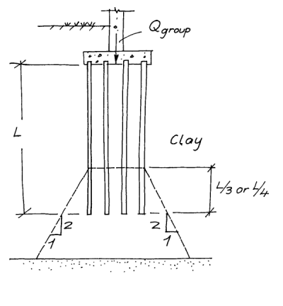
The 2:1 method is the only method taught in Soils in Construction. It is generally used with shallow foundations, but can also be applied to pile groups in clay, as shown at the right. It’s simplicity and reasonable accuracy has brought it acceptance, and further information on it can be found in the Soils and Foundations Reference Manual. The concept has also been applied to pile toes, and you can see this in STADYN Wave Equation Program 10: Effective Hyperbolic Strain-Softened Shear Modulus for Driven Piles in Clay.

Academic Issues, Geotechnical Engineering

Specific Surfaces of Soil Materials

Posted on 24 April 20248 August 2026 by Don Warrington

One concept that appears at the end of Chapter 1 of Soils in Construction is that of the specific surfaces of soil materials, including data from Lambe and Whitman’s classic text Soil Mechanics. Additional information on this topic can be found in Tsytovich, which is reproduced below. (Tsytovich refers to this as “unit surface area,” but the concept is the same.)

A factor of importance in the evaluation of the properties of solid soil particles is their mineral composition. Thus, some minerals, such as quartz and feldspar, interact only slightly with the surrounding water, whereas other minerals, for instance, montmorillonite, can interact substantially more actively and in a different way. The smaller the particles of a soil, the greater their unit surface area (per cm³ or per gram) and the larger the number of centres of interaction with the surrounding water and in contacts between solid particles proper. For instance, particles of kaolin (a clay mineral) have a unit surface area of 10 m²/g, whereas those of montmorillonite have a very large unit surface area of 800 m²/g, which inevitably affects the properties of natural soils containing particles of montmorillonite. The presence of particles of mica (which are very slippery and have only a negligible shear resistance) has an essential effect on the physical properties of the soils containing such particles; this circumstance must always be taken into account.

It can be shown that, for spherical particles, the unit surface area can be computed using the formula

$A_{us} = \frac{3}{r \rho}$

where r is the radius of the particle and $\rho$ is the density of the material. We thus can see that, for a uniform particle density (which is nearly the case for inorganic soil particles) the unit surface area is inversely proportional to the radius or diameter of the particle. Thus smaller particles have a higher unit surface area and larger particles a lower one. The units, as presented by Tsytovich and others, are tricky, as they combine SI or MKS units with CGS ones.

Academic Issues, Geotechnical Engineering

The “Why” and “What” of Soils in Construction

Posted on 22 April 202422 April 2024 by Don Warrington

Anyone familiar with the history of geotechnical engineering is aware that its development can, to some extent, be tracked with the development of its textbooks. Early textbooks tended to be vague and empirical in nature. With new books more theory is found, especially after the works of Terzaghi, Peck, Tschebotarioff and Taylor. By the early 1970’s there was a large selection of textbooks for the undergraduate instructor to choose from in the topics of soil mechanics, foundations or books that featured both.

This selection, which peaked with the end of the “Golden Age” of geotechnical engineering, has thinned considerably, as it has with most textbooks. Soils in Construction made its debut in 1974, right in the middle of the last burst of activity in the field. So why has this textbook endured when so many others have fallen by the wayside?

The answer is simple: it wasn’t aimed at undergraduate civil engineering students but at construction management ones, and in that respect it was far enough ahead of its time to endure but no so far as to die before its time would come.

When I started my career in the 1970’s, people with geotechnical knowledge working for contractors were a rare breed. This is not to say that such people had not taken their place; the likes of Lazarus White comes to mind. But most contractors–especially small and medium size firms, firms which frequently specialised in one or more aspects of geotechnical construction–did not have on staff people with a working knowledge of applied geotechnical theory.

Contractors were not alone in this lack. State DOT’s were likewise short of people with this type of understanding, and they had large sums of public money entrusted to them. The FHWA saw the need to address this issue, and the Soils and Foundations Reference Manual was the result of that effort. Although it can be used in a college setting (I have done this in my Soil Mechanics and Foundation Design and Analysis courses) it takes a lot of work, more work than most academics are used to putting into an undergraduate course.

Soils in Construction is the answer to this dilemma. It is geared towards construction management students whose mathematical level may not be up to that of their engineering counterparts. (But…I always told my students that the only calculus they’d get in my courses is if they didn’t brush their teeth; even for them it is the nature of basic geotechnical engineering.) It enables them to grasp the basics of the application of soil mechanics to practical problems, including temporary works, whose engineering is frequently overlooked but which is often vital for the successful completion of the permanent works to follow.

With this the authors commend this work to our readers, hoping that it will result in more successful geotechnical projects for contractor, owner and engineer alike.