Academic Issues – Page 4 – vulcanhammer.net

Academic Issues, Geotechnical Engineering, Soil Mechanics

Getting to the Legacy of B.K. Hough and his Settlement Method

Posted on 14 March 202413 June 2025 by Don Warrington

Note: since I first wrote this, more information has come to light (for me at least,) which is contained in the post Closing the Loop (or at least trying to) on Hough’s Settlement Method.

Last year I posted The Sorry State of Compression Coefficients where I a) gave a brief summary of earlier posts on consolidation settlement and b)showed that there was more than one way to express them. An example of the “alternative” (for geotechs in some countries it’s the accepted way) compression coefficient is “Hough’s Method” which is featured in both the Soils and Foundations Reference Manual and the Shallow Foundations manual. Hough’s Method, however, is for cohesionless soils. Why, you ask, can methods usually associated with cohesive soils be applied to cohesionless ones? Because consolidation settlement methods using the logarithmic difference of pressure reflect the fact that the elastic (or shear) modulus of a soil increases as the void ratio/porosity of the material decreases, which I discuss in From Elasticity to Consolidation Settlement: Resolving the Issue of Jean-Louis Briaud’s “Pet Peeve”.

In this post I will attempt to do two things:

The method as presented in the above references has been described as too conservative, i.e., the settlements predicted are too large. I will attempt to explain this and perhaps offer a solution based on Hough’s own works.
Discuss the whole business of bearing capacity vs. settlement failure in shallow foundations, which was perhaps the greatest legacy of Hough’s work and remains an important issue in geotechnical engineering today.

Bearing Capacity vs. Settlement

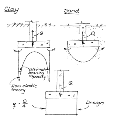
Terzaghi’s solution (or more accurately his adaptation of Prandtl’s punching shear theory) of the bearing capacity problems was one in a number of solutions that became “reference standard” in geotechnical engineering.

We were regaled with photos of Canadian grain elevators on their side to show that bearing capacity failure was the first thing we should look for in shallow foundation design. Terzaghi’s formula was so highly regarded that for many years it was fashionable for introductory geotechnical courses to require students to learn both Terzaghi’s method and the subsequent improvements/extensions of that method by researchers such as Meyerhof, Vesic, Brinch Hansen, etc..

Up until that time shallow foundations were generally designed using what we call “presumptive bearing capacities” based on soil types and foundation configurations. These were enshrined in the building codes of the day. They were generally purely empirical in nature, as was most of geotech in the era before Terzaghi and his contemporaries. They had one advantage however: because they were derived from actual performance, be it ever so crude, they included the effects of soil settlement under load.

Like any other engineering material, only on a larger basis (because their elastic/shear moduli were several orders of magnitude lower than more conventional materials) soil is deformable under load. That deformation not only allows the foundation to deflect under load, it also affects the failure surfaces as they develop. The latter reality became apparent and so we have the modification of the bearing capacity for punching and local shear. It should be noted that Terzaghi and Peck were well aware of the problem of settlement, and included provision for it in their classic 1948 textbook Soil Mechanics in Engineering Practice.

One possible solution was to use elastic theory for the initial settlement. The implementation of that is discussed in Analytical Boussinesq Solutions for Strip, Square and Rectangular Loads. It is even possible to develop a lower bound solution for the bearing capacity problem, as was discussed in Lower and Upper Bound Solutions for Bearing Capacity. The problem with this is twofold. The first is that the lower bound solution assumes that the footing is a purely flexible foundation, which is not really true with this type of foundation. The second is that, if we went to the other extreme and assumed a purely rigid foundation, by elastic theory the stresses at the corners is infinite for any load. (This is conventionally attributed to foundations in cohesive soil, but it can be shown to be true by elastic theory.)

Hough’s Settlement Method

Hough presented his settlement method in his 1959 ASCE paper. He starts by presenting a graph similar to the following, which illustrates the transition from small, elastic displacement to large inelastic ones:

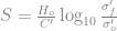
The solution is in the form (similar to that presented in Verruijt) of

$S=\frac{H_{o}}{C'} \log_{10} \frac{\sigma'_f}{\sigma'_o}$

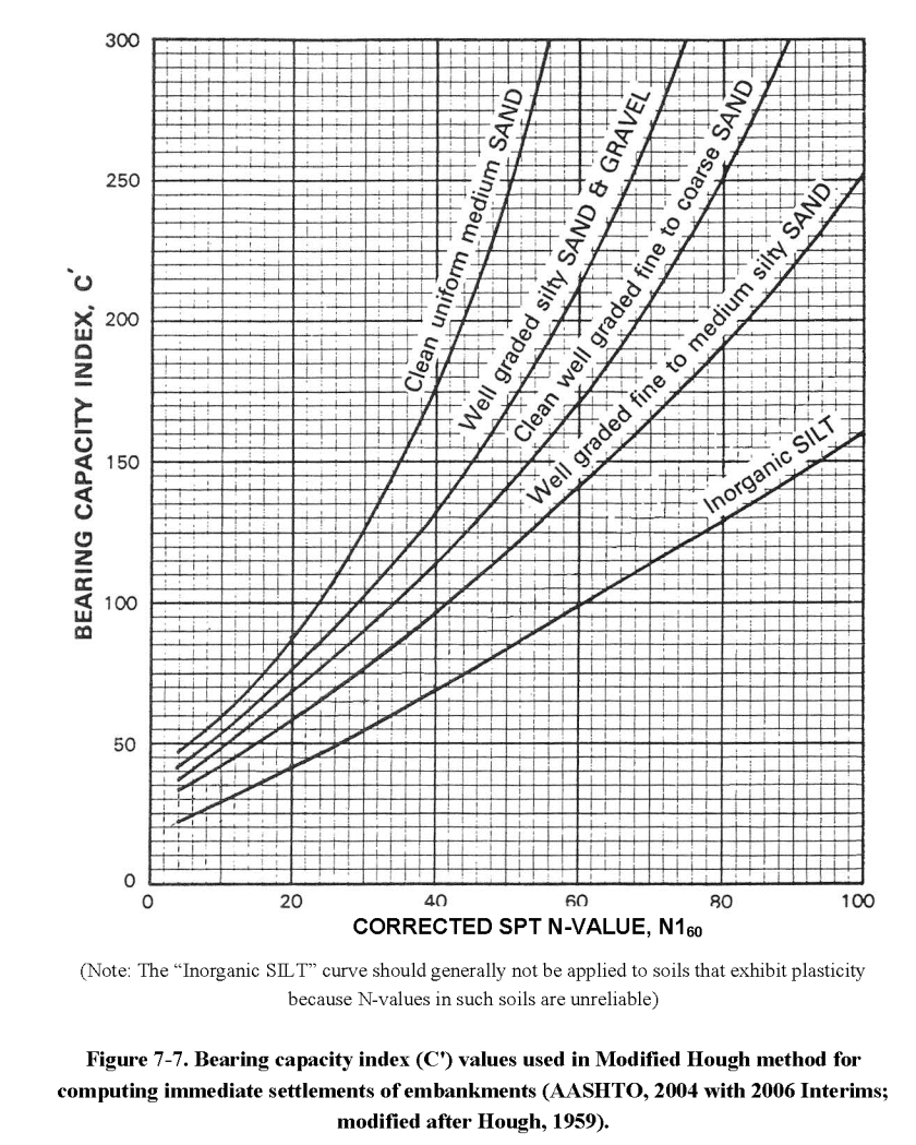
The coefficient $C'$ is determined using a chart which is below.

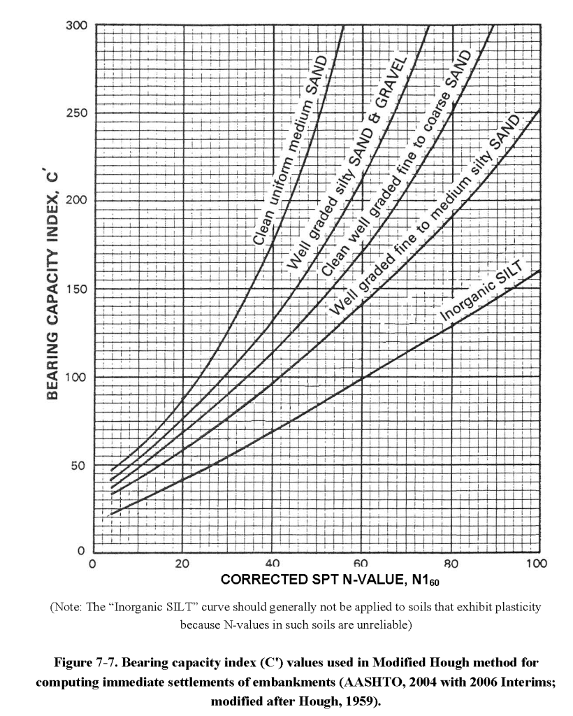
The chart itself is basically the same as the one in Hough (1959,) but now things get complicated.

In Shallow Foundations we are informed of the following:

Cheney and Chassie (2000) recommend that the SPT blowcounts be corrected for overburden pressure before correlating the N-values to the bearing capacity index,
C′. An overburden correction by Bazaraa (1967) was recommended by Cheney and Chassie (2000). Since that time, many researchers have studied the effect of overburden stress on the SPT N-value, largely in support of liquefaction hazard assessment procedures. Recent consensus by the 1996 and 1998 National Center for Earthquake Engineering Research (NCEER) (Youd et al., 2001) concluded that the correction proposed by Liao & Whitman (1986) (shown in Figure 5-18) could be used for routine engineering applications. Therefore, the correction by Liao & Whitman is included here as part of the Hough procedure, in particular because it is easy to calculate and can be used without charts in simple computation spreadsheets.

The basic problem with this is that Hough himself never mentions any kind of correction for the variations of the SPT tests, overburden or otherwise, and that in modifying Hough’s Method we run the risk of making some assumptions that may not be applicable.

The idea of using the SPT tests, even with shallow foundations in cohesionless soils such as the ones Hough is concerned about, is admirable on the face because undisturbed samples of these soils are hard to obtain in normal soil testing. The problem with SPT tests–which were coming into acceptance when Hough presented his original method–is that their variations in both configuration and those induced by the overburden are significant. It wasn’t until the 1980’s that this was “formally” sorted out with the correction system that we have today.

With our current method we have two stages of correction. The first stage is for variations in the configuration of the split spoon, the effect of the rod and borehole, and most importantly the efficiency of the hammer itself. The second is for the overburden. In both his original paper and the presentation of the method in the Second Edition of his textbook Basic Soils Engineering (1969,) Hough does not delve into either of these.

The whole point of the N₆₀ correction (the first series) was to harmonise the results to a single mechanical standard, and one that was generally attained “back in the day” so that empirical methods such as Hough’s could be used today. We could assume that Hough’s value are at least N₆₀ values, although we’re not guaranteed of that due to the lack of supporting data.

The business of overburden correction brings up Bazaraa (1967.) At this point credit needs to be given where credit is due: Bazaraa had the thankless task of sorting out the settlement methods which were current in his day, and that task included dealing with the variations of the SPT method. Since his overburden correction method was originally used with Hough’s Method and then changed, let us compare the two. We start be defining

$p_{norm} = \frac{\sigma'_o}{p_{atm}}$

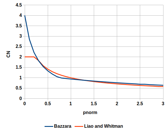
The two correction factors $C_N$ for overburden are shown below.

Except for the region where Liao and Whitman is “flat topped” the two are reasonably close, and so substituting Liao and Whitman’s correction is legitimate, assuming it should be used at all.

It should be noted, however, that Bazaraa’s objective is not to correct Hough’s method, which he did not do: it was to provide a new method of estimating settlements in cohesionless soils, and to advance Terzaghi and Peck’s 1948 method. So we are still “up in the air” about how to apply all of this to Hough’s Method.

If the overburden stress is less than the standard atmospheric pressure (approx. 2 ksf) then the N value used will be increased, the C’ values will likewise increase, and the estimated settlement will decrease, which may be more accurate but moves away from conservatism. If the opposite is true then the result will be more conservative. For shallow foundations such as Hough’s Method the lower overburden stresses will be more of a factor (depending upon the depth D.) At this point it is not clear to me (at least) that including an overburden correction is really significant given the other unsolved problems that exist with this method.

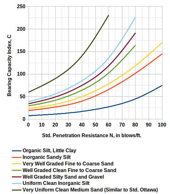
One further complicating factor is that, in the aforementioned Second Edition of Basic Soils Engineering, Hough presents a new chart (again with no explanation of correction of any kind) which is redrawn as follows:

Some trend line work results in a correlation in this form:

$C = A \exp^{BN}$

where the coefficients A and B are below.

Soil Type	A	B
Organic Silt, Little Clay	7.22	0.0229
Inorganic Sandy Silt	18.28	0.021
Very Well Graded Fine to Coarse Sand	22.86	0.0203
Well Graded Clean Fine to Coarse Sand	28.22	0.0216
Well Graded Silty Sand and Gravel	32.85	0.0216
Uniform Clean Inorganic Silt	37.02	0.0221
Very Uniform Clean Medium Sand (Similar to Std. Ottawa)	58.66	0.0225

It should be noted that, where the curves are directly comparable with Hough (1959), they tend to be lower, i.e., the values of C are less. This would increase settlement and thus conservatism. At this point perhaps we should consider Hough’s Methods in the plural rather than the singular.

Beyond Hough’s Method

To start this part consider this, from NAVAC DM 7.1:

We have the conventional C_c based on either liquid limit, initial void ratio or water content. Hough is represented here as well; however, these correlations are for cohesive soils. Hough himself had a broader application for these.

In the Second Edition of Basic Soils Engineering, he presents a function to compute C_c as follows:

$C_c = a(e_0 - b)$

He also establishes a relationship between correlations based on liquid limit and those on void ratio, but getting to that is for another time.

In any case he presents values for this equation which are tabulated below, and include both cohesionless and cohesive soils.

	a	b*
Uniform cohesionless Material (C_u < 2)
Clean Gravel	0.05	0.5
Coarse Sand	0.06
Medium Sand	0.07
Fine Sand	0.08
Inorganic Silt	0.1
Well-graded, cohesionless soil
Silty sand and gravel	0.09	0.2
Clean, coarse to fine sand	0.12	0.35
Coarse to fine silty sand	0.15	0.25
Sandy silt (inorganic)	0.18	0.25
Inorganic, cohesive soil
Silt, some clay; silty clay; clay	0.29	0.27
Organic, fine-grained soil
Organic silt, little clay	0.35	0.5

*The value of the constant b should be taken as e_min whenever the latter is known or can conveniently be determined. Otherwise, use tabulated values as a rough estimate.

From here we can use the well-tried “C_c” formulae (which would include preconsolidated soils) to estimate settlement. This opens up a new vista for using conventional consolidation settlement theory to estimate the settlements of cohesionless soils.

To return to our original objectives, settlement and bearing capacity are, in the process of failure, two sides of the same thing. It is also worth noting that most foundations fail in settlement, although the failure isn’t as “spectacular” as bearing capacity.

The only way to treat them together is to use a method that can combines both phenomena, and finite element methods are capable of doing that. However our profession has been uncomfortable with “black box” methods such as these, although they really apply the same laws we use to formulate closed form solutions. In that respect they have value, and to apply methods such as Hough’s to cohesionless soils with better calibration of the constants would be a good step forward.

References

Bazaraa, A.R.S. (1967). “Use of the Standard Penetration Test for Estimating Settlements of Shallow Foundations on Sand,” Ph.D. Thesis presented to University of Illinois, Urbana.
Hough, B.K. (1959). “Compressibilty as the Basis for Soil Bearing Value,” Journal of the Soil Mechanics and Foundations Division, ASCE, Vol. 85, Part 2.
Hough, B.K. (1969). Basic Soils Engineering. Second Edition. New York: Ronald Press Company.
Kimmerling, R.E. (2002). Shallow Foundations: Geotechnical Engineering Circular No. 6. FHWA-SA-02-054. Washington, DC: Federal Highway Administration.
Terzaghi, K. and Peck, R. (1948). Soil Mechanics in Engineering, 1st Ed., John Wiley & Sons.

Academic Issues, Geotechnical Engineering

Bengt Broms RIP

Posted on 12 March 2024 by Don Warrington

We may be a little late to the announcement but we regret to inform you of the following:

Professor Bengt Baltzar Broms, Stockholm, Sweden, passed away at the age of 95. He is survived by his wife Carina and children Erik, Karin, and Peter.

Bengt Broms was a leading figure in Swedish and International Geotechnology and Foundation Engineering. He is mourned by many colleagues around the world, especially his former doctoral students, whom he mentored with exceptional expertise and generous advice.

For this site, in addition to his research work his contribution has been the numerous drawings that he posted online back in the late 1990’s/early 2000’s, in the early years of both this site and of my teaching at the University of Tennessee at Chattanooga. I still find them very useful and certainly better than my own “chicken scratchings.”

Memory eternal.

Academic Issues, Geotechnical Engineering

A Simplified Method to Design Cantilever Gravity Walls

Posted on 6 October 202316 June 2025 by Don Warrington

On this site we feature the U.S. Army Corps of Engineers publication Retaining and Flood Walls, which details the design of several types of retaining walls. As it was published a good while back, it details the design of these walls using hand calculations. Sometimes these can get tedious, especially when the aptly named “trial wedge” solutions are employed.

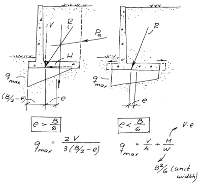
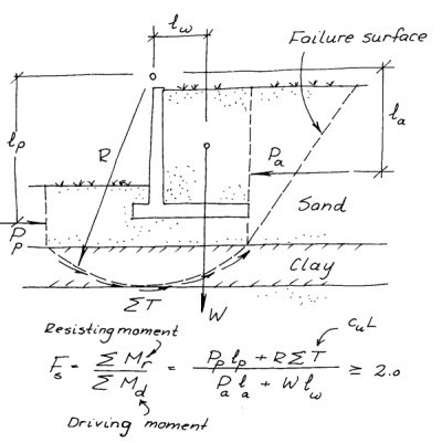
These days it’s more likely that a computer solution–be it a true finite element analysis or simply the automation of those tedious hand calculations–is used to finalise the design of a retaining wall. An example of such an analysis is shown above, and addresses in particular an issue that gets the short shrift in classical retaining wall analysis of any kind: global stability failure. An idea of a hand solution to this problem is shown at the right. Global stability failures still happen and are generally disastrous; beyond a conventional slope their analysis is fairly complex.

But in the meanwhile, what do we do to verify that we’ve got it right with a computer solution? Or what can we do to start with a reasonable design that we can refine with numerical analysis? Back in the “slide rule era” we used quick, “back of the envelope” methods to design things, and we can use them today both to get started and to gain a basic understanding of the elements of the design.

In this case we’re going to discuss the design of a cantilever retaining wall, an example of which is shown below.

The methodology is based on the aforementioned Retaining and Flood Walls and the example (which is a little clearer description of same) comes from Appendix A of Seismic Analysis of Cantilever Retaining Walls, Phase I. I’ve modified it in a couple of spots and will detail those modifications as we go.

The example we’ll look at is below. We need to design this wall to prevent failure against three events: sliding, overturning and bearing capacity failure.

Defining the Geometry, Weights and Centres of Gravity

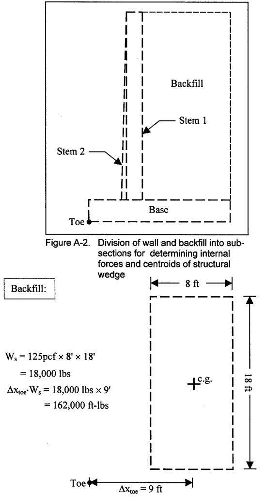
Our datum/coordinate origin is at the toe, which is convenient since we assume that the overturning moment is computed around the toe. Since this is a cantilever/gravity wall, the weight of the wall is part of the resistance force and moment. Included with that is the backfill that is trapped behind the wall (shown above.)

We start by dividing up the wall into sections, each of which has a weight and a centre of gravity. The first section we take up is the backfill, which is a simple rectangle shown above.

At this point we need to make one correction to the Corps’ work: the weights and moments are in pounds per unit length of wall and ft-pounds per unit length of wall, respectively. Leaving those per unit length designations is a common shortcut among practitioners but is confusing for students, who frequently find the unit length concept difficult to grasp at first. The weight of the backfill is properly 18,000 lbs/ft of wall and the moment around the toe ((clockwise) is 162,000 ft-lbs/ft of wall.

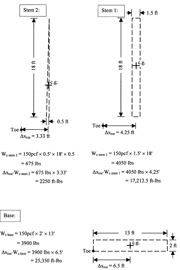
Computing the weights and moments of the various sections of the wall itself yields the following results.

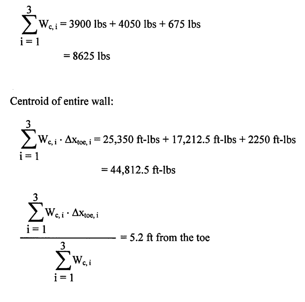
Taking all of this information and processing it yields the total weight, total moment around the toe, and moment arm around the toe:

Since most engineers have learned their statics via vectors, a review of Vector Statics and “Old Coot” Statics: An Example and What is a Resultant in Geotechnical Engineering? may be in order.

The Shear Mobilisation Factor

Now comes the tricky part: in retaining wall design, we traditionally define the factor of safety as

$FS = \frac{F_{resisting}}{F_{driving}}$ (1)

Where the “F” values can be forces or moments and FS is the factor of safety. Sometimes this is not the optimal way of applying factors to account for uncertainties, especially when we get to LRFD. Another approach is either to increase the driving force or reduce the resisting force. We do the latter with sheet piling (where there there are earth forces to resist) but here we’ll to the former. To make this happen we first define a shear mobilisation factor (SMF) thus

$SMF = \frac{\tan \phi'_{mob}}{\tan \phi'}$ (2)

The value of $\phi'_{mob}$ can be computed thus:

$\phi'_{mob} = \tan^{-1}(SMF tan \phi')$ (3)

For this problem, assuming SMF = 2/3 and φ’ = 35°, by substitution φ’_mob = 25°. We will discuss the effect of cohesion later.

Now we turn to computing the force of the soil behind the wall on the wall.

We note the following:

Rankine theory is used. Methods shown in both Retaining and Flood Walls and the Soils and Foundations Reference Manual use Coulomb and/or log-spiral for these computations. The problem with this is that the value of wall friction δ is sometimes difficult to determine without data or experience, and in reality most of this pressure bears on soil, not the wall. So Rankine is easier to start with, and is more conservative.
The backfill is level, the formula for Ka only applies in that case. We will discuss sloping backfill below.
Note that φ’_mob (not φ’ ) is being used to compute the soil force.

Analysing Sliding and the Location of the Resultant/Overturning

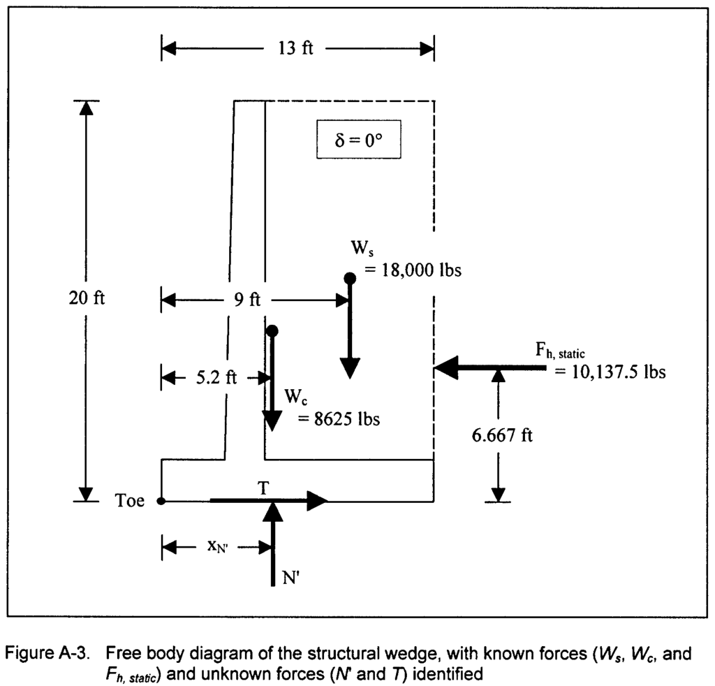
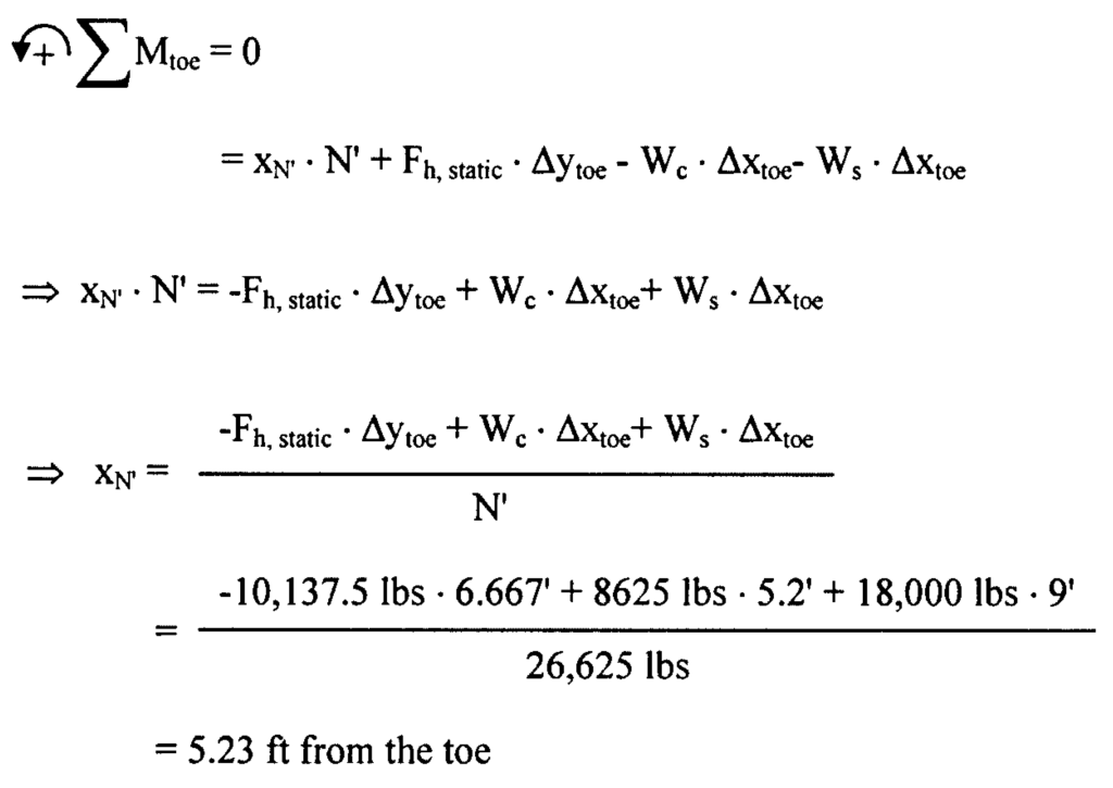
At this point we can compute the forces on the base (both the forces T’ and N’ and the location of the resultant x_N’,) which are shown below.

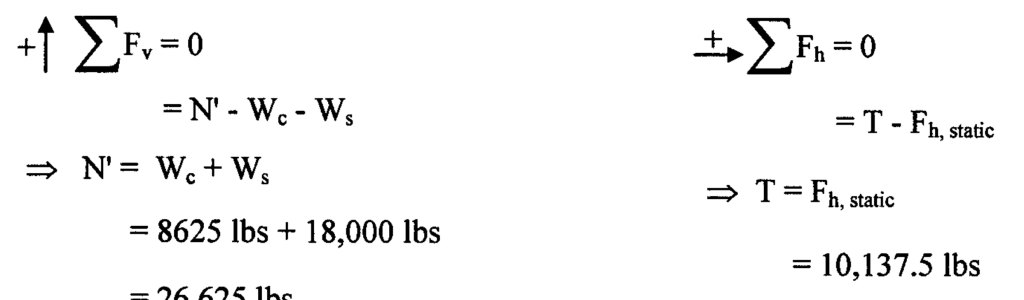
The calculations are shown below.

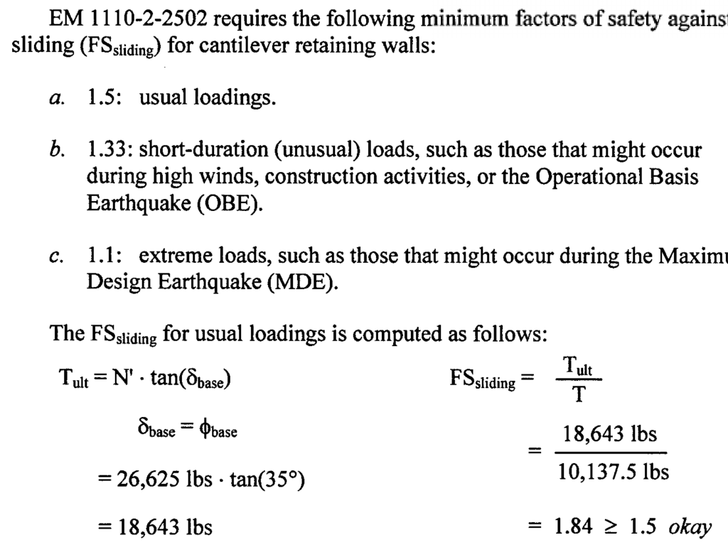
Turning to the sliding problem, the driving force is the earth pressure force and the resisting force is the maximum Coulomb friction of the base/soil interface. In this case the value of δ is equated to the unmodified value of φ’, although that isn’t always the case. (The basis for this is that there is a thin layer of backfill sand under the wall, under which is a different foundation soil.) We then apply Equation (1) and determine the factor of safety against sliding, which checks out against the Corps criteria.

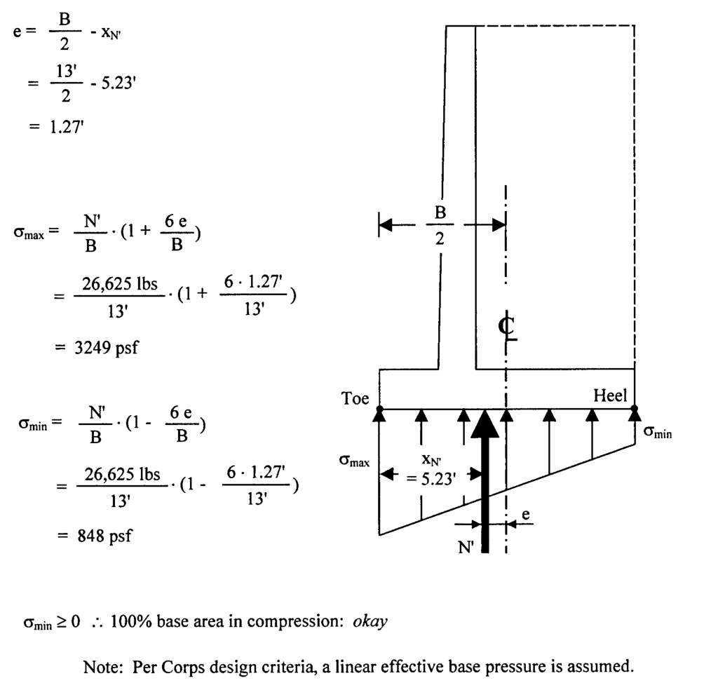
Knowing the location and magnitude of the resultant, we compute the maximum and minimum pressures on the base. Since both pressures are compressive, the resultant is in the middle third, and thus we can proceed with the base design.

One thing that is missing from this analysis is a specific analysis for overturning. In this case we make a common assumption that, as long as the resultant force of the wall is within the kern and there are no negative pressures on the base, overturning will not be experienced. It is certainly possible to do an explicit overturning analysis to check this result.

Bearing Capacity Analysis

With the wall’s sliding and overturning established, we turn to the bearing capacity analysis of the base. The complete bearing capacity equation, from the Soils and Foundations Reference Manual (with modification,) is

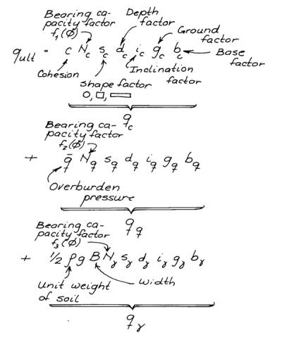
$q_{ult}=s_{c}b_{c}l_{c}cN_{c}+s_{q}b_{q}l_{q}C_{wq}q_{o}N_{q}+\frac{1}{2}s_{\gamma}b_{\gamma}l_{\gamma}C_{w\gamma}\gamma B_{f}N_{\gamma}$ (4)

where

q_ult = ultimate unit upper bound bearing capacity
s_c, s_γ and s_q = shape correction factors. These are unity in this case since it is a continuous foundation (generally the case with retaining walls)
b_c , b_γ and b_q = base inclination correction factors (unity in this case since the foundation is level)
C_wγ and C_wq are groundwater correction factors (unity in this case since groundwater isn’t an issue, a rare event with retaining and especially flood walls)
I_c, I_γ and I_q = load inclination factors, discussed below
N_c , N_q and N_γ are bearing capacity factors that are a function of the friction angle of the soil. N_c , N_q and N_γ are shown in the table below. These are handled differently when a slope is present. They are given in the Soils and Foundations Reference Manual. There is a general consensus for N_c and N_q but not N_γ. In this case we will use Vesić’s values for it, following AASHTO/FHWA practice. For this case the base soil φ’ = 40° we have N_c = 75.3, N_q = 64.2 and N_γ = 109.4
B_f = Base width of the foundation. In this case, with an eccentrically loaded foundation, this must be reduced to the equivalent foundation width by the formula B’_f = B_f – 2e = 13 – (2)(1.27) = 10.46’.
q₀ = overburden pressure on the base from the dredge (low) side of the wall. For walls such as this we neglect all effects of this, both any potential passive lateral pressure and overburden pressure.
c = cohesion of the soil = 0
- Because of this and the previous point, we can neglect the first two terms of Equation (4) and only concern ourselves with the last one.

Load inclination is the result of two perpendicular loads acting on the base of the foundation. It is illustrated in the sketch at the left.

The load inclination factors are given as follows:

$l_{c}=l_{q}=\left(1-\frac{\delta'}{90\textdegree}\right)^{2}$ (5a)

$l_{\gamma}=\left(1-\frac{\delta'}{\phi'}\right)^{2}$ (5b)

where the load inclination angle is given as follows

$\delta' = \tan^{-1}\frac{T}{N'}$ (6)

Substituting yields 𝞭’ = tan^-1 (10,137.5 lbs/26,625 lbs) = 20.8°. The friction angle of the base soil proper is 𝟇 = 40°. Substituting into Equation (5b) yields l_𝞬 = (1-20.8/40)² = 0.23. We can neglect the factors for Equation (5a) as those terms do not apply to this situation, but for completeness l_c = l_q = (1-20.8/90)² = 0.591.

Making all relevant substitutions:

q_ult = (0.5)(1)(1)(0.23)(1)(10.46)(125)(109.4) = 16,450 psf
Q_ult = q_ult B_f = (16,450)(10.46) = 172,067 lbs. = 172 kips
N = 26,625 lbs
FS = Q_ult/N = 172067/26625 = 6.46 (acceptable)

Settlement Analysis

Settlement of retaining wall is an important topic, as settlement of walls and levees has led to overtopping (as we found out the hard way during Hurricane Katrina.) Instead of picking a method and doing it “by hand,” we will use the USACOE software package CSANDSET, developed by Virginia Knowles. To accomplish this we need to do the following:

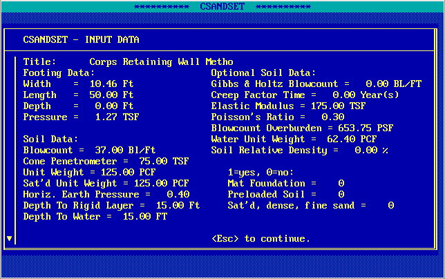
The foundation with we use is the reduced foundation width, or B’_f = B_f – 2e = 13 – (2)(1.27) = 10.46’.
The normal load is N = 26,625 lbs.
The unit load on the foundation is thus 26625/(2000*10.46)=1.27 tsf (the units used by the program.)
We assume a length of 50′; this puts the L/B > 10, which is an assumption for continuous foundations.

The input data is shown in the screenshot below.

The SPT and CPT are taken from “typical” values as they were not given in the problem statement. The option data is generated by the program. The horizontal (at-rest) earth pressure is Jaky’s Equation for normally consolidated soils.

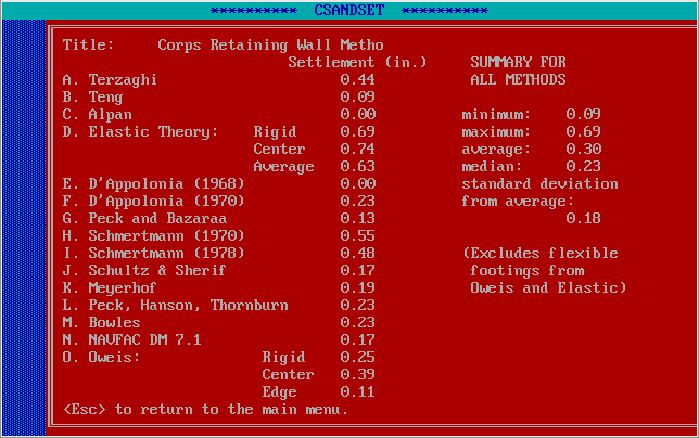
The solutions the program gives are as follows:

The various methods are described in the program documentation. Schmertmann’s Method is given a full description in Foundation Design and Analysis: Shallow Foundations, Settlement. Elastic methods are treated in Soil Mechanics: Elastic Solutions to Soil Deflections and Stresses and related posts. It is interesting to note the wide variance in results; this is typical of geotechnical methods in a state of flux, and can also be applied to bearing capacity of driven piles.

The supplemental data generated by the program is at the end of the post.

Dealing with Sloping Backfill

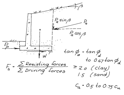
The example problem above has a level backfill. Sloping backfills–usually positive (up from the wall,) occasionally negative, are common with retaining walls. The problem of the sloping backfill is illustrated at the right.

Without going into the actual solution of the problem using a sloping backfill, the following changes must be made in order to accommodate the effects of this condition:

The Rankine equation for sloping backfill needs to be applied. This can be found in the post Rankine and Coulomb Earth Pressure Coefficients. The coefficient computed is actually Coulomb theory applied without wall friction; the differences between this and “extended Rankine” theory for sloping backfill are discussed in the post on the coefficients.
An additional region needs to be defined with the soil below the sloping backfill (assuming it’s positive) as shown in the diagram below.
The length a of this region is already defined. The length b is given by the equation b = a tan (β). That length is important in a) computing the weight of the region and b) computing the additional length of the height the soil bears on the wall, or H + b.
The backfill force must be separated into horizontal and vertical components, as shown in the diagram above. The vertical component actually increases both the weight on the foundation and the resisting moment of the weight.

Assuming a β = 10° and applying φ’_mob = 25°, with the geometry shown we note the following:

With the two angles shown, K_a = 0.462, which is higher than the level backfill value.
The value of b = (8)(tan(10°))=1.41′. This means that the total height is 20 + 1.41 = 21.41′.
The lateral pressure at the base is (0.462)(21.41)(125) = 1236.5 psf.
The total lateral force on the wall F_h is (1236.4)(21.41)/2 = 13,236 lb/ft of wall. The resultant of that force is 21.41/3 = 7.14′ above the base of the foundation.
That lateral force has a horizontal component of (13236)(cos((10°)) = 13,035 lb/ft and a vertical component of (13236)(sin(10°)) = 2298 lb/ft. The latter has a moment arm of 13′ from the toe.
The area added by the sloping backfill has a weight W_ba = (125)(8)(1.41)/2 = 705 lb/ft. Its centroid is located 5 + (2)(8)/3 = 10.3′ from the toe.

We will leave working out the effects of this backfill slope to the reader.

The Shear Mobilisation Factor (SMF) and Cohesive Soils

If we have soils with cohesion in the backfill, the cohesion should be modified in a similar way to the friction angle thus:

$c' = c \times SMF$ (7)

A more complete treatment of the SMF is given in Retaining and Flood Walls.

Academic Issues

My View of Student Evaluations

Posted on 21 September 2023 by Don Warrington

One thing any academic does (except those at grand institutions where they get to have someone else do it for them) is evaluate students through grading. Most institutions afford students the opportunity to retaliate through the faculty evaluation system in place. That usually takes places at the end of the term, although my institution now had mid-term evaluations in place.

Student evaluations of faculty always take me back to this incident in my own undergraduate saga:

One of the things that the Mechanical Engineering department required* its majors to take was Logic, which was offered by the Philosophy Department. Most of the engineers did pretty well in this course, which was doubtless a source of secret frustration to liberal arts’ professors.

One day I went up to pick up a test from the professor. The professor looked at the grade, noted that I had nearly aced it, looked at me, and exclaimed, “You’re not as dumb as you look!”

The purpose of student evaluations of me is to determine whether they agree with my Logic teacher’s opinion or not.

*Originally posted here. Since then I discovered that there was another option available, but my advisor at the time did not avail me of that choice.

Academic Issues, Deep Foundations

Comments on “Using the Impulse–Response Pile Data for Soil Characterization”

Posted on 5 August 20235 August 2023 by Don Warrington

It’s citation time again; this paper, authored by Heeyong Huh, Heedong Goh, Jun Won Kang, Stijn François and Loukas F. Kallivokas, cites both Closed Form Solution of the Wave Equation for Piles and Improved Methods for Forward and Inverse Solution of the Wave Equation for Piles. It is available here. The abstract is as follows:

The impulse–response (IR) test is the most commonly used field procedure for assessing the structural integrity of piles embedded in soil. The IR test uses the response of the pile to waves induced by an impulse load applied at the pile head in order to assess the condition of the pile. However, due to the contact between the pile and the soil, the recorded response at the pile head carries information not only about the pile, but about the soil as well, thus creating the as-yet-unexplored opportunity to characterize the properties of the surrounding soil. In effect, such dual use of the IR test data renders piles into probes for characterizing the near-surface soil deposits and/or soil erosion along the pile–soil interface. In this article, we discuss a systematic full-waveform-based inversion methodology that allows imaging of the soil surrounding a pile using conventional IR test data. We adopt a heterogeneous Winkler model to account for the effect of the soil on the pile’s response, and the pile’s end is assumed to be elastically supported, thus also accounting for the underlying soil. We appeal to a partial differential equation (PDE)-constrained-optimization approach, where we seek to minimize the misfit between the recorded time-domain response at the pile head (the IR data), and the response due to trial distributions of the spatially varying soil stiffness, subject to the coupled pile–soil wave propagation physics. We report numerical experiments involving layered soil profiles for piles founded on either soft or stiff soil, where the inversion methodology successfully characterizes the soil.

Over the years I have been looking at many different aspects of the problem of pile dynamics, which includes both prediction of drivability of piles and the inverse problem of estimating the static resistance of piles based on their performance during driving. In the course of working with all of this many ideas have come to mind; two of those are as follows:

Is it possible to use the model (or something like it) in Closed Form Solution of the Wave Equation for Piles for the inverse method? My experience with Improved Methods for Forward and Inverse Solution of the Wave Equation for Piles and its progeny informed me that managing the inverse method in a full FEA model including pile and soil was difficult and getting past uniqueness issues (which have plagued pile dynamics from the start) was next to impossible.
Is it possible to use the pile hammer as a geotechnical sounding tool to determine the properties of soil layers into which the pile is being driven? In Improved Methods for Forward and Inverse Solution of the Wave Equation for Piles the soil at any given point was defined by the “Mohr-Coulomb triple” (unit weight, internal friction angle and cohesion) along with other properties, which is the point for most soil testing. The inverse method returned those properties.

The present paper does some interesting things to get to those solutions but ultimately doesn’t quite get to reaching a solution to these problems.

The Strong Point

Probably the strongest point of the paper is the entire mathematical presentation, from the development of the method to its execution. It shows computational proficiency of a high order. For example, it is the first time in pile dynamics that I have seen the use of the conjugate gradient technique. As the product of a PhD program with a heavy emphasis on computational fluid mechanics, this technique was well familiar to me (along with GMRES, which was the method of choice for my colleagues.) One of the challenges the geotechnical industry faces moving forward is the proper application of numerical techniques to geotechnical problems which are non-linear in ways which are unknown in other fields. We have people who are specialists with the geomechanics and people who are specialists in numerical methods, but few are those who are proficient in both.

One thing I would like to mention is that my use of a polytope method–which had many drawbacks–was driven by the difficulties in optimising geotechnical problems. Those difficulties are caused largely by the existence of false minima and maxima in the solution. It is why we still see, for example, grid optimisation used for slope stability problems: the use of, say a Newton’s Method type of optimisation may easily result in finding a false minimum. Although I think the author’s techniques have great promise of solving these problems, it is something they will have to watch for moving forward.

The Soil Property Issue

Probably the greatest weakness of the paper is the way soil properties are characterised.

Let us first consider the system model presented in Closed Form Solution of the Wave Equation for Piles, shown below.

Simplified Hammer-Pile-Soil System (from Warrington (1997))

In this diagram the ram mass M impacts the cushion with a velocity V_o. There are several stiffnesses and damping coefficients k and c respectively. The accessory has a mass of m. The pile has an acoustic speed c, an impedance Z and a geometry ratio r_g. For inverse analysis the hammer, cushion and driving accessory can be deleted and a force F(t) and velocity V(t) (both a function of time) substituted at the pile head.

The equation of motion u(x,t), which is a function of both the distance from the pile head x and time t, is given by the equation

${c}^{2}{\frac {\partial ^{2}}{\partial {x}^{2}}}u(x,t)={\frac {\partial ^{2}}{\partial {t}^{2}}}u(x,t)+au(x,t)+2\,b{\frac {\partial }{\partial t}}u(x,t)$ (1)

The variables a and b are stiffness and damping related coefficients which are related to k and c by geometric and material property considerations, as discussed in Closed Form Solution of the Wave Equation for Piles.

Although the present paper allows for k(x), the one major difference between the governing equation presented above and the one in the paper is the omission of damping by the latter. (This omission is also repeated at the pile toe.) The soil damping is for the most part a representation of the propagation of wave energy from the pile as it is dynamically loaded. It is impossible to avoid in one form or another. First derivatives like that are always a danger in problems such as this. One way to get around that is to redistribute the damping into the spring and mass terms using Rayleigh damping. This is very frequency dependent and can be tricky to accurately apply; however, if it can be done successfully (and the authors’ note of wavespeed changes with soil interaction may be part of the solution) it would bypass the problems created by the first derivative. (The same comments regarding the shaft also apply at the toe, where an additional mass would have to be applied to achieve Rayleigh damping.)

But that doesn’t address what is, in some ways, the more serious issue: applying a linear model to a very non-linear problem. Concentrating on the shaft resistance, let us begin by noting the results in Estimating Load-Deflection Characteristics for the Shaft Resistance of Piles Using Hyperbolic Strain Softening, and stipulating that, even with hyperbolic stress-strain considerations, up to the time of separation between the shaft and the soil the load-deflection relationship is essentially linear. This study showed that, for the specific case in question, the geometric nonlinearity of the deflecting soil around the shaft and the material nonlinearlity of the soil offset each other to a large degree. Obviously more study needs to be done but this is a start.

Having said that, let us look at a diagram I have used and modified over the years:

At zero strain we have the small strain elastic or shear modulus. As strain increases, if we use a linear model for load-deflection the only way the model can simulate that kind of response is to do some kind of “secant modulus” estimate. What this means is that the elastic modulus/shear modulus/spring constant is strain dependent, which will vary with loading condition (to put it in classical geotechnical terms, to what extent the shaft resistance is mobilised.) It is also worth noting that this mobilisation is not identical in static and dynamic testing, even on the same pile.

Based on all of this, it is difficult to see how the results of the inverse method can be used to accurately characterise the load-deflection characteristics of the pile, let alone the properties of the soil.

I should note that quite a few of my comments in Comments on “Fictitious soil pile model for dynamic analysis of pipe piles under high-strain conditions” apply to this situation as well. This linearity problem is a major reason why I never have attempted to use the model in Closed Form Solution of the Wave Equation for Piles as a “full-up” inverse method.

Conclusion

This paper is an interesting study of the problem at hand. While some significant advances have been done in the numerical treatment of the problem, the physics of the pile-soil system need to be re-examined and improved.