Academic Issues – Page 5 – vulcanhammer.net

Comments on “Fictitious soil pile model for dynamic analysis of pipe piles under high-strain conditions”

Posted on 3 August 20235 August 2023 by Don Warrington

Once again I find myself cited, this time in this paper by Yuan TU , M.H. El Naggar , Kuihua Wang , Wenbing WU , and Juntao WU. The citation comes from my paper “A New Type of Wave Equation Program,” documenting the development of the ZWAVE computer program. The abstract of this paper is as follows:

A fictitious soil pile (FSP) model is developed to simulate the behavior of pipe piles with soil plugs undergoing high-strain dynamic impact loading. The developed model simulates the base soil with a fictitious hollow pile fully filled with a soil plug extending at a cone angle from the pile toe to the bedrock. The friction on the outside and inside of the pile walls is distinguished using different shaft models, and the propagation of stress waves in the base soil and soil plug is considered. The motions of the pile−soil system are solved by discretizing them into spring-mass model based on the finite difference method. Comparisons of the predictions of the proposed model and conventional numerical models, as well as measurements for pipe piles in field tests subjected to impact loading, validate the accuracy of the proposed model. A parametric analysis is conducted to illustrate the influence of the model parameters on the pile dynamic response. Finally, the effective length of the FSP is proposed to approximate the affected soil zone below the pipe pile toe, and some guidance is provided for the selection of the model parameters.

The topic is an interesting one which I have touched on over the years. It seems to me that their characterisation of the model as “novel” may be a bit of a stretch but their implementation of it is very interesting.

What is a Fictitious Pile Model?

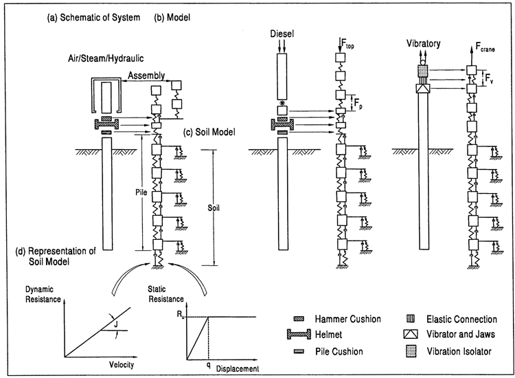
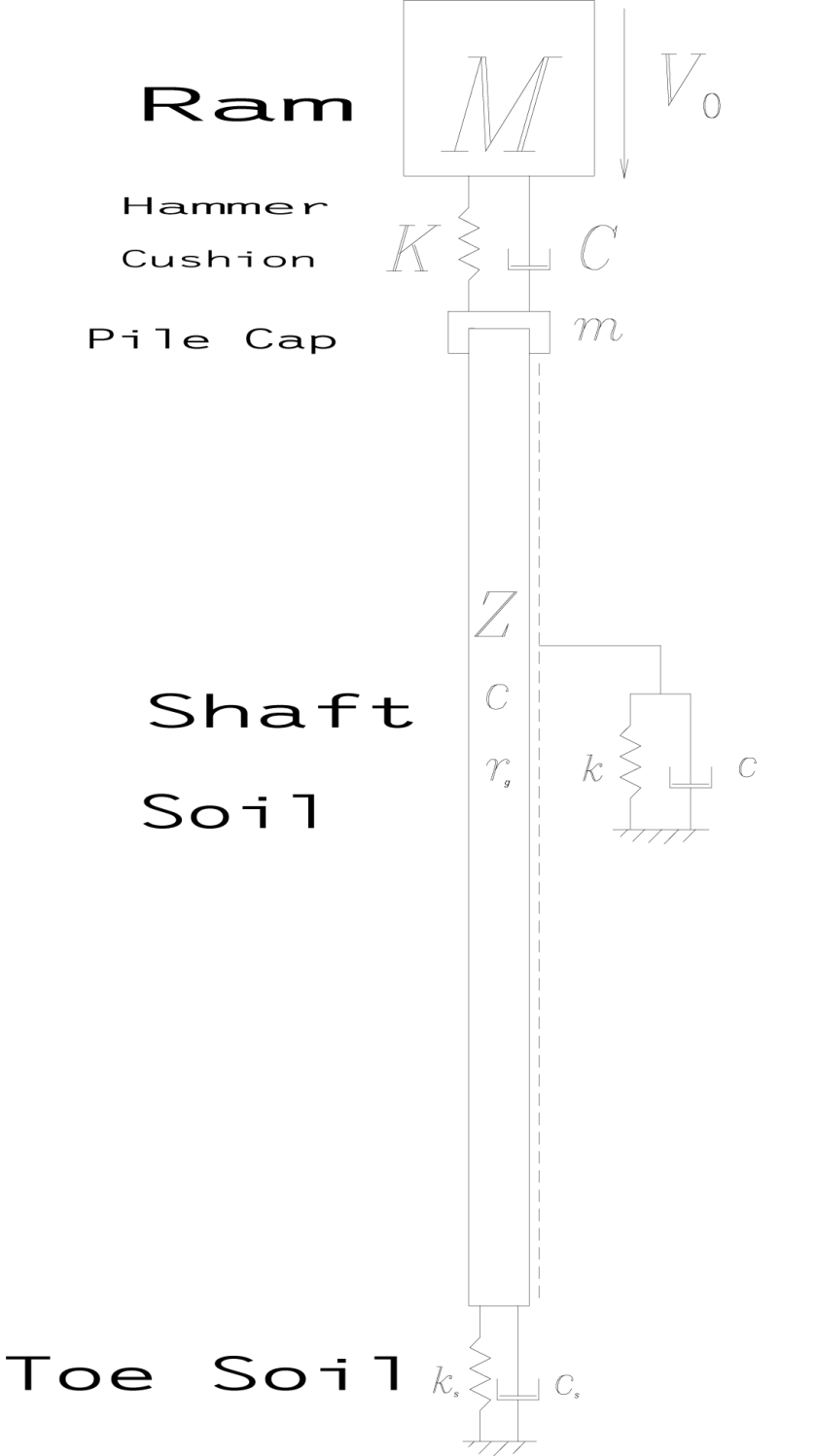
Most of us in the driven pile industry are familiar with the one-dimensional wave equation, which divides up the pile into discrete segments/elements and by doing so models the distributed mass and elasticity (or plasticity) or the system, such as is shown in Figure 1, from the Design and Construction of Driven Pile Foundations, 2016 Edition:

Figure 1 One-Dimensional Wave Equation Method Diagram (from Soils and Foundations Reference Manual)

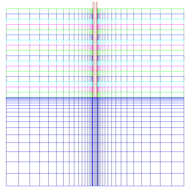
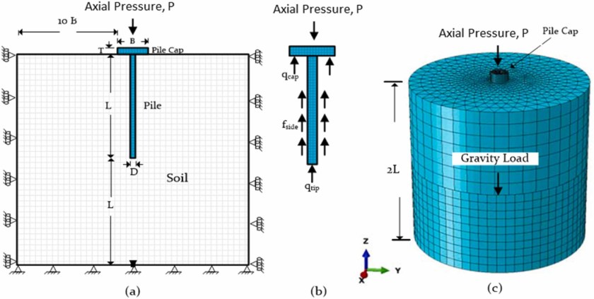
An advance of this is the use of two- or three-dimensional elements in a finite element scheme, such as was featured in the earlier post Comments on “3D FE analysis of bored pile- pile cap interaction in sandy soils under axial compression- parametric study” and was analysed extensively in my dissertation Improved Methods for Forward and Inverse Solution of the Wave Equation for Piles. A cross section of that model is shown in Figure 2, from Inverse Analysis of Driven Pile Capacity in Sands:

Figure 2. Cross-Section of Finite-Element Model for Pile and Soil (from Warrington (2020))

Note that the pile, which is in red, is basically a one-dimensional string of elements with distributed mass and elasticity. It’s worth noting, however, that using two- (or three- for that matter) dimensional elements enables the element to have a non-uniform stress distribution which would reflect the effect of the soil resistance, but let us set this last point aside.

Such a model as shown above models both the shaft friction along the side of the pile and the toe resistance under the end of the pile. It has been customary over the years, however, for researchers and practitioners alike to model this resistance in a rheological way. This has been easier with the shaft than with the toe, because of the complexities of the dynamic elasto-plastic response of the soil at the toe and the difficulties of establishing failure surfaces in the soil has led to many solutions of the problem.

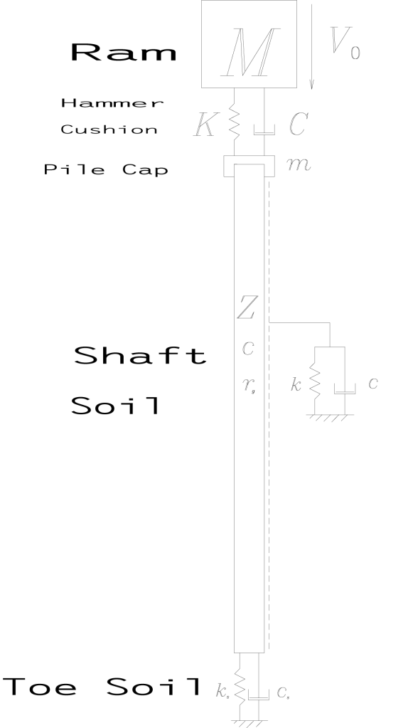
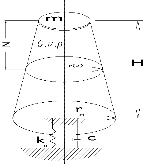
One of those is to construct a fictitious pile under the toe which, instead of the straight sides we usually (but not always) see with piles, has a conical shape, so as the distance from the toe increases the size of the fictitious pile likewise increases.

Figure 3. Fictitious Pile Model for the Pile Toe (from Holeyman (1988); Warring-
ton (1997))

The first proposal of this came from Holeyman (1988) and was discussed in Closed Form Solution of the Wave Equation for Piles and more recently in the paper STADYN Wave Equation Program 10: Effective Hyperbolic Strain-Softened Shear Modulus for Driven Piles in Clay. A diagram of this is shown in Figure 3. Although the model is generally done (as is the case in the models in Figure 1) with discrete elements, it can be modeled continuously. The paper under consideration did so using finite elements. A problem that occupied this researchers and those of the paper under consideration is the value of H, which does not have an “obvious” solution from the physics of the problem.

In the work under review, in addition to using finite elements the authors made two important improvements to the model shown in Figure 3:

They added a “shaft” resistance along the side of the fictitious piles.
They put a hole in the centre of the fictitious pile to assist in simulating the soil plug, which was one of the main goals of the study. Soil plugging is a difficult phenomenon in open-ended piles, and although we’ve made some progress in modelling it we still have a long way to go.

Some Comments on the Study Itself

The authors used ABAQUS to model both piles. This is a code which has been applied to geotechnical problems for at least thirty years, so it has a long track record. Having started from “scratch” with Improved Methods for Forward and Inverse Solution of the Wave Equation for Piles, I can attest that using a software package saves a great deal of time and effort, in addition to making graphical presentation of the results a good deal simpler. Having said that, if anyone has an ambition to use FEA to replace, say, GRLWEAP or CAPWAP, they’ll have to either a) pay licensing fees to a cut down “engine” from an established package like ABAQUS or b) use an open source alternative.

At the start of the study they make the following statement:

Open-ended pipe piles are increasingly used worldwide as foundations for both land and offshore structures [1,2]; therefore, the characterization of pipe pile capacity and behavior under static and dynamic loading conditions has gained much attention in recent years [3–5].

Open ended pipe piles have been used for much longer that this paragraph would imply, as this whole series will show. Getting them in the ground was much of the impetus for the TTI wave equation program, and the lateral loads they withstood were much of the push behind the development of p-y methods. And that was in the 1960’s and 1970’s.

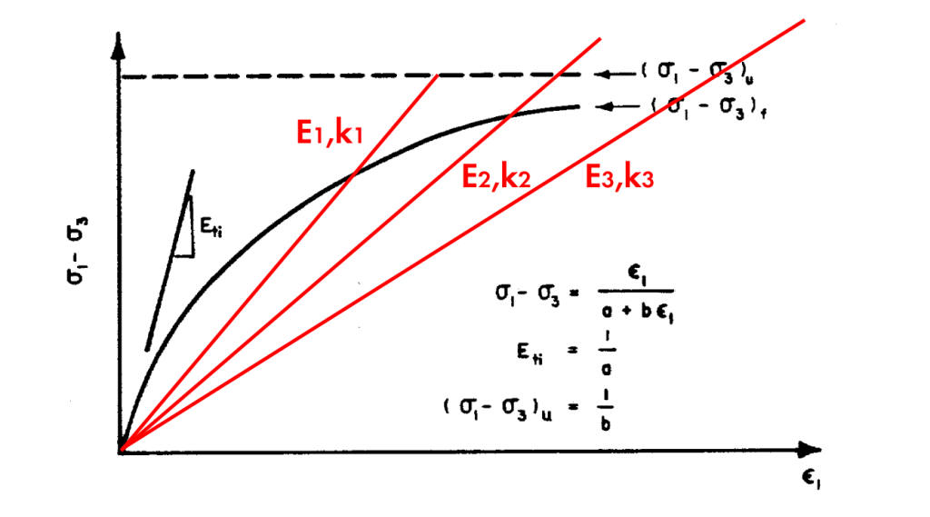
The soil model they use is a cross between a elastic-purely plastic model and a hyperbolic soil model. Reconciling the two has been a preoccupation of this site since Relating Hyperbolic and Elastic-Plastic Soil Stress-Strain Models: A More Complete Treatment. Although the model they use certainly takes into consideration hyperbolic strain softening, I’m not convinced that their assumption that the rebound runs along the small-strain modulus of elasticity is valid. On the other hand I’m not sure what the best way out of this dilemma is; hyperbolic soil modelling hasn’t been as thorough in analysing the stress-strain characteristics of soil during rebound as it has been in doing so during loading.

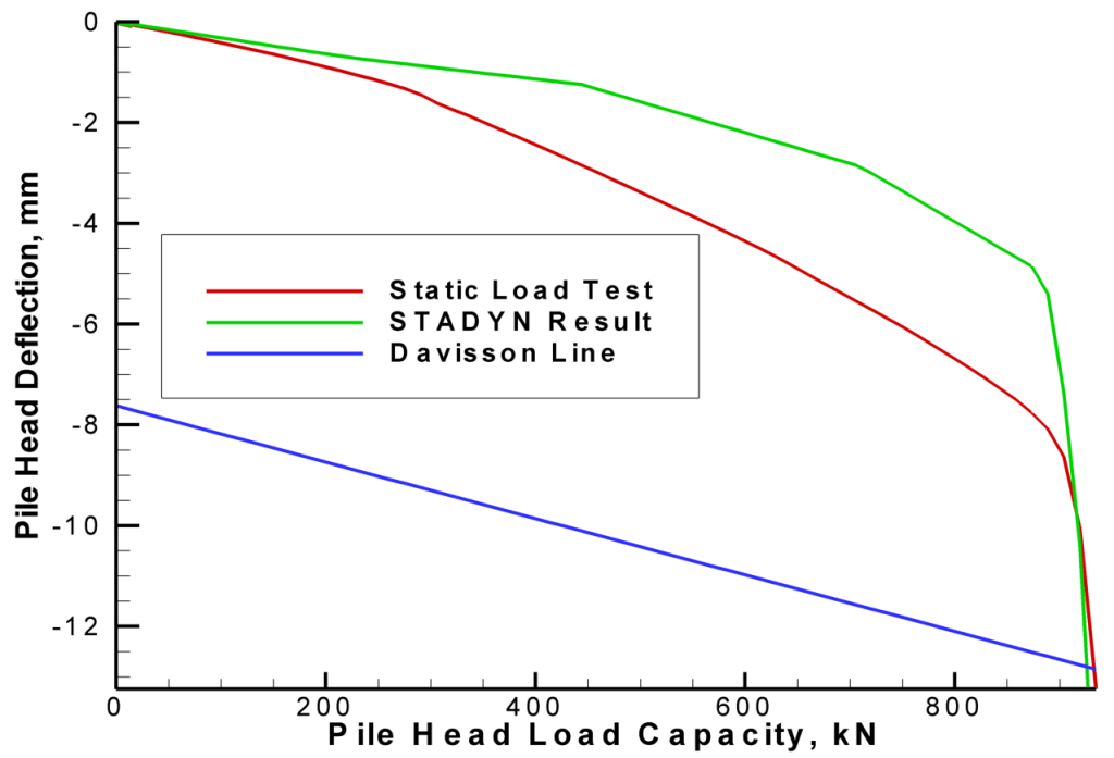
One thing I noticed is the variance between the static load test results and that shown in the model. That’s not unexpected; I’ve encountered this difficulty, as you can see from this figure in STADYN Wave Equation Program 10: Effective Hyperbolic Strain-Softened Shear Modulus for Driven Piles in Clay:

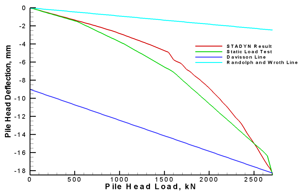
On the other hand, it’s possible to get a closer result, as is seen in Application of the STADYN Program to Analyze Piles Driven Into Sand:

The basic problem is twofold:

Although the relationship between the shear modulus of soils and the void ratio or porosity is well established, the coefficient used to determine the former from the latter is subject to uncertainty.
The static and dynamic shear moduli of soils is different, which is an issue in pile dynamics that has not been adequately explored.

Conclusion

The paper is an excellent step forward, and the model presented has a great deal of potential in pile dynamics. It may be easier to use such a model than a full axisymmetric or 3D model to obtain the inverse solution to the problem, but many of the issues discussed here–such as the angle and depth of the fictitious pile cone and the shear moduli of the soils in question–need better resolution.

As far as the plugging issue is concerned, any advance in this is welcome, although I am inclined to think that a model which simulates the full, blow-by-blow installation of the pile with the formation of the plug, will ultimately be the best solution of the problem.

Comments on “3D FE analysis of bored pile- pile cap interaction in sandy soils under axial compression- parametric study”

Posted on 26 July 2023 by Don Warrington

As always I was gratified to be cited in the recent paper “3D FE analysis of bored pile- pile cap interaction in sandy soils under axial compression- parametric study,” by Faisal I. Shalabi, Mohammad U. Saleem, Hisham J. Qureshi, Md Arifuzzaman, Kaffayatullah Khan, and Muhammad M. Rahman. It is an interesting study of the topic at hand. Some comments are in order:

Although the citation is of Closed Form Solution of the Wave Equation for Piles, the work Improved Methods for Forward and Inverse Solution of the Wave Equation for Piles is really closer to the methodology shown in the paper, both in terms of the 3D FEA used (well, I took a shortcut and used axisymmetric 2D analysis) and to the use of Mohr-Coulomb theory for the analysis, which I discuss in An Overview of Mohr-Coulomb Failure Theory and Elasto-Perfect Plasticity with Mohr-Coulomb Failure. Mohr-Coulomb is still viable for many applications, especially with sands.
One especially interesting aspect of this study was the inclusion of a pile cap. The problem is similar to the the one I discuss in my post When Semi-Infinite Spaces Aren’t, and When Foundations are Neither Rigid Nor Flexible, where the foundation is neither perfectly flexible relative to the soil nor perfectly rigid. Although in this study the foundation rigidity is not varied, the soil’s is, and as is the case in elastic theory as the soil becomes less rigid the relative rigidity of the foundation increases, the soil stresses relative to the foundation towards the edge of the foundation likewise increase. This Fall I plan to include that elastic theory in my discussion of mat foundations here: Foundation Design and Analysis: Shallow Foundations, Other Topics.
I noted a drop in the shaft friction just before the toe, followed by an increase down to the toe itself. The interaction between pile, soil and shaft friction for deep foundations is a complicated one. The toe creates failure surfaces in the soil that are certainly there–and it is reasonable to assume that they affect the shaft friction near the toe as well–but they are not exactly like those generated in shallow foundations, something which has complicated toe resistance calculations for a long time. The relative uniformity of the unit toe resistance makes sense based on failure theories going back to at least Vesić’s work in the early 1970’s. One thing that bored piles do not have to consider is the effects of advancement due to impact which, as Mark Randolph’s work has shown, almost show a “leading edge” effect.

It is my opinion that 3D FEA will ultimately be our best tool for estimating the load/settlement characteristics of deep foundations–bored or driven, static or dynamic–and this paper is a step forward in that regard.

Academic Issues, Geotechnical Engineering

The Sorry State of Compression Coefficients

Posted on 27 May 2023 by Don Warrington

I’ve dealt with the issue of consolidation extensively since my first post on the subject, From Elasticity to Consolidation Settlement: Resolving the Issue of Jean-Louis Briaud’s “Pet Peeve”. His problem was the lack of relationship between the way we handle consolidation settlement vs. elastic settlement. In this post I plan to look at a different problem, i.e. the way we express the relationship between soil pressure and consolidation settlement, or settlement by rearrangement of the particles.

Up to now…

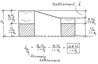
Let’s start with the diagram at the right, from Broms (as will be the case with the graphics we use.) Soil is made up of a combination of soil particles and voids between them. The voids can be filled with air, water or (God forbid) something else. For saturated soils water, for practical purposes, fills all of the voids.

In any case, for illustrative purposes we can “melt” the solids into a continuous solid and leave the rest as a void. We assume that the solids do not compress during the application of pressure and thus their volume is constant. From the first state (on the left) to the second state (on the right) additional pressure is applied. All the change of the volume must take place in the void; the equation at the bottom is based purely on the geometry, where $H_o$ is the height of the layer being compressed, $e_o$ is the initial void ratio of the soil, $\Delta e$ is the change in void ratio during compression, and $\delta_p$ is the primary settlement of the soil.

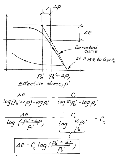
Unfortunately, as discussed elsewhere on this site, the relationship between the increase in pressure and the settlement/change in the volume of the voids isn’t linear but (empirically) logarithmic. That is shown in the graphic on the left; once the pressures get past the ambient effective stress, the settlement takes places according to the relationship shown at the bottom of the graphic. Here $C_c$ is the compression coefficient, $p'_o$ is the effective stress, and $\Delta p$ is the change in pressure on the soil at a given point.

Combining the two equations in the two graphics yields the “accepted” form of the consolidation settlement equation for normally consolidated soils, thus

$\delta_p = \frac{C_c H_o}{1+e_o} \log_{10} (\frac{p'_o + \Delta p}{p'_o})$ (1)

To this deceptively absolute state of affairs Verruijt has the following objections:

We should be using natural logarithms instead of common ones. Common logarithms date from the days when engineers used logarithmic and semi-logarithmic paper, determining $C_c$ graphically. The compression coefficients would be changed by multiplying or dividing (depending on the form, more on that shortly) by a factor of 2.3. In an era of spreadsheets and MATLAB, natural logarithms would make more sense (and reduce student mistakes,) but I don’t see that changing.
We should use the strain rather than the void ratio. Actually, as Verruijt points out, this is done in Continental Europe. In the U.S. and Scandinavia, void ratio is used as the parameter of deflection. To change this would require a change in the compression coefficient, and that leads to…
…his preferred form of the compression equation, which would look like

$\epsilon = \frac{1}{C_{10}} \log_{10} (\frac{p'_o + \Delta p}{p'_o})$ (2)

where $C_{10}$ is another form of the compression coefficient. (Well, actually, he’d prefer natural logarithms, but as I said let’s put that aside.)

Multiplying both sides of Equation (2) by $H_o$ gives us

$\delta_p = \frac{H_o}{C_{10}} \log_{10} (\frac{p'_o + \Delta p}{p'_o})$ (3)

The two compression coefficients are related as follows:

$\frac{1}{C_{10}} = \frac{C_c}{1+e_o}$ (4)

Actually a variant of Equation (4) finds its way into American practice in Hough’s Method for sands, which is described in the Soils and Foundations Reference Manual.

Enter NAVFAC DM 7.1

The “New” NAVFAC DM 7.1 (Soil Mechanics) is an excellent compendium of the current state of geotechnical practice relating to soil mechanics. In the process of discussing consolidation settlement, it highlights some recent changes that promise to add to the confusion described above.

For normally consolidated soils, Equations (1) and (3) are written as follows

$\delta_p = C_{\epsilon c} H_o \log_{10} (\frac{p'_o + \Delta p}{p'_o})$ (5)

where $C_{\epsilon c}$ is the modified compression index. This means that Equation (4) can be expanded as follows:

$\frac{1}{C_{10}} = \frac{C_c}{1+e_o} = C_{\epsilon c}$ (6)

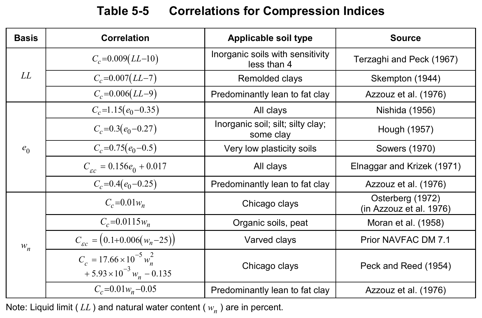
Whether we can dispense with the initial void ratio is a separate topic. Assuming that we can, what we have is a situation with three different compression coefficients, all designated with some form of $C_x$ , and none of them the same. (If we threw in natural logarithms, we’d have six.) The potential for confusion is evident, no where than when two of the three coefficients end up in the same table:

And Secondary Compression…

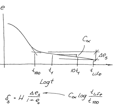
Secondary compression has had the problem for much longer. If we look at Graphic 3 on the right, we see that we have a secondary compression coefficient $C_{\alpha}$ . The presentation is a little hard to follow but the secondary compression equation is

$\delta_s = \frac{C_{\alpha}H_o}{1+e_o} \log_{10}\frac{t_{life}}{t_{100}}$ (7)

where $\delta_s$ is the amount of secondary compression, $C_{\alpha}$ is the coefficient of secondary compression, $t_{life}$ is the life of the structure and $t_{100}$ is the time at which 100% of primary compression has taken place. (Of course that’s a source of confusion in itself because, in theory, 100% primary compression is never achieved, something that buffaloed many of my students on a test last semester.)

However, as NAVFAC DM 7.1 points out, we can also write this as

$\delta_s = C_{e \alpha}H_o \log_{10}\frac{t_{life}}{t_{100}}$ (8)

where the modified secondary compression coefficient is

$C_{e \alpha} = \frac{C_{\alpha}H_o}{1+e_o}$ (9)

So what is to be done?

My advise to students and practitioners alike is to be vigilant and careful. Make sure you understand which coefficient is being called for. For software, make sure you completely understand which coefficient is being used by the software; otherwise, you will have the classic “garbage in/garbage out” result. Verruijt hoped that we would come to uniform practice but we can’t wait for this; we have to get our work done, and we need to do it carefully.

Academic Issues, Civil Engineering

Floating or Compensated Foundations

Posted on 5 April 20235 April 2023 by Don Warrington

One type of foundation that needs some explanation are floating or compensated foundations. Since they are sometimes referred to as “floating,” some fluid mechanics background is in order.

Fluid Mechanics

For ships to float, they obey Archimedes’ Law, where the weight of the ship is equal to the weight of water displaced by the hull of the ship. This is more thoroughly explained in my handout Buoyancy and Stability: An Introduction. I also go through all this in this video:

If the hull of the ship is rectangular, it’s also possible to compute the upward force of the water–which equals the downward force of the weight–by multiplying the hydrostatic pressure by the plan area of the ship, as is shown below. As the ship settles further and further into the water, the hydrostatic pressure increases until equilibrium is reached.

Illustrating Water Pressure Increasing in Proportion to the Draught

This last will be useful when we consider soils because, although box shaped ships are not so common, box shaped buildings and foundations are.

Turning to buildings, soils are an intermediate material between pure fluids and solids. Some are obviously more intermediate than others, but in softer soils they are more “fluid-like.” Let us consider the multi-storey building at the right.

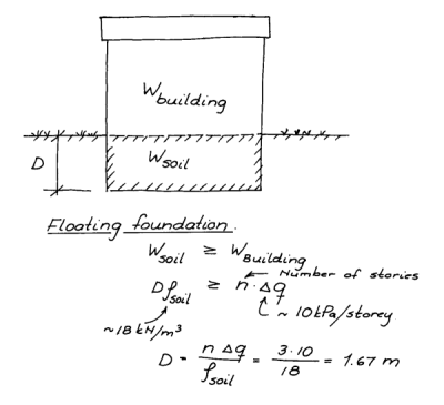
If we consider that the soil acts as a fluid, then for the building to “float” in the soil the weight of the soil displaced must be greater than or equal to the weight of the building. The difference between ships and buildings is twofold. One, it is possible for a building to weigh less than the weight of the soil displaced and not get shoved upward until equilibrium is reached. The second is that, frequently, we use a “per unit area” approach to balance the equation and come up with the “draught” D of the building.

In this case we have a three-storey building where each storey has a unit weight of 10 kPa, or 10 kN per square metre of area. Multiplying the number of storeys n by the unit weight Δq yields 30 kPa. The soil weight is 18 kN/m³, or otherwise put the displaced soil exerts an “upward force” of 18 kPa/m of depth. Dividing the downward pressure by the unit weight yields a foundation depth/draught D = 1.67 m.

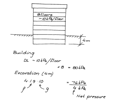
At this point it is worth noting that, depending upon the properties of the soil, it is not always necessary for the soil displaced to equal in weight to the building, but can be less. This is because soils, unlike fluids, have shear strength when not moving, an issue I discuss in my monograph Variations in Viscosity. An illustration of this is at the left.

Here we have a building with eight storeys and 10 kPa/floor, for a total pressure of 80 kPa. On the soil side we have a unit weight of 19 kN/m³ (after eliminating those pesky kilogram force units) and a foundation depth of 4 m, which results in an upward pressure of 76 kPa. The difference between the two is 4 kPa, not much but still enough to reduce the depth of the basement if the soil were a true fluid.

It’s first worth noting that an alternative way to look at the problem is that we are computing the total stress of the foundation at the base and then comparing it with the downward pressure of the building. That works for box like structures such as we are dealing with. If we have a more complex structure such as is shown at the right, we will have to adjust our strategy.

Beyond that, soils are routinely called upon to handle normal and shear stresses induced by the pressure exerted on the foundation. How well they do this is at the core of geotechnical foundation design. We must consider whether foundations will fail in bearing capacity, settlement or both. Bearing capacity is not as great of a problem with “large” structures such as mat foundations as it is with spread footings. Settlement, whether elastic or consolidation, is a major issue, and is something else that separates soils from fluids: rearrangement of the particles during volume change of the soil.

How much net pressure that is permissible is something that needs to be considered once it is established. Nevertheless, it is possible to use the soil’s own weight to help balance and support the structure during its useful life.

Note: graphics are from Bengt Broms, and more of these can be found in the post Bengt Broms Geotechnical Slides.

Academic Issues, Civil Engineering

When Semi-Infinite Spaces Aren’t, and When Foundations are Neither Rigid Nor Flexible

Posted on 4 April 202329 April 2023 by Don Warrington

In our posts Analytical Boussinesq Solutions for Strip, Square and Rectangular Loads and Going Around in Circles for Rigid and Flexible Foundations we discussed foundations on an elastic, homogeneous half-space, mostly purely flexible. In the latter post we ventured into rigid foundations but stuck with the semi-infinite spaces. In this post we’re going to explore cases where either one of the other or both of these aren’t true.

Some Review: Purely Rigid Foundations

In Going Around in Circles for Rigid and Flexible Foundations we looked at stress distributions under circles (and strip loads for that matter.) The results can be summarised graphically below, from Tsytovich (1976).

Figure 1. Isobars in Soil under Foundations a)absolutely rigid foundation, b)flexible foundation (from Tsytovich (1976))

View (a) shows a point load on a rigid foundation; it could be a distributed one too, as long as the load is concentric. In any case at the corners the vertical stress is infinite. In the real world one would expect the soil to go plastic long before that and the stresses to redistribute themselves, but we’ll stick with pure elasticity for the moment.

View (b) shows a distributed load on a flexible foundation. At the interface between the foundation and the soil the vertical stress is the load p, and it decreases the further you get away from the foundation. The strip load version of this is used to find the lower bound solution for bearing capacity in Lower and Upper Bound Solutions for Bearing Capacity.

This is the state of affairs for foundations which are either perfectly flexible or perfectly rigid. The truth is that neither one of these extreme approximations is really true. This is illustrated in the figure below.

Figures 2. Diagrams of contact pressures a) under an absolutely rigid foundation, b) under foundations of various flexibilities. (From Tsytovich (1976))

View (a) shows the rigid foundation with the stresses at the base of the foundation as they would be in elastic theory (solid line) and those with some “real world” plasticity thrown in (dashed line.)

If the rigid foundation is circular, for a semi-infinite, elastic homogeneous space, the stress distribution is as follows:

$\sigma_{z}=\frac{p}{2\sqrt{1-\left(\frac{x}{r}\right)^{2}}}$ (1)

where

$\sigma_z =$ vertical stress in soil
$p =$ uniform pressure on foundation. With rigid foundations we can have a point load P and obtain the same result as long as the load is at the centroid of the foundation
$x =$ distance from centroid
$r =$ radius of foundation

The relationship between a distributed load and a point load at the centroid is

$P = p \pi r^2$ (2)

For a rigid strip foundation,

$\sigma_{z}=\frac{2p}{\pi\sqrt{1-\left(\frac{2y}{b}\right)^{2}}}$ (3)

where

$y =$ distance from centreline of strip load
$b =$ width of foundations

If we define, as is done in Figure 1, the half width of the foundation as

$b_1 = \frac{b}{2}$ (4)

then Equation (3) becomes

$\sigma_{z}=\frac{2p}{\pi\sqrt{1-\left(\frac{y}{b_1}\right)^{2}}}$ (5)

The line load can be computed as follows:

$P = p b$ (6)

View (b) shows a foundation with varying flexibility and the effect that has on stress distribution at the base. The flexibility of the foundation is described by the variable $\Gamma$ . We’ll discuss how that’s calculated later but $\Gamma$ is a measure of the flexibility of the foundation.

$\Gamma = 0$ is a totally inflexible (rigid) foundation
$\Gamma = \infty$ is a totally flexible foundation.

Before we get to that, let’s take a look at the other problem, that of a non-semi-infinite half space.

Non-Infinite Spaces and Flexible Foundations

We’ll start with this problem, which is a progression from what we saw in Analytical Boussinesq Solutions for Strip, Square and Rectangular Loads and Going Around in Circles for Rigid and Flexible Foundations. Unfortunately the state of some of our usual sources forced us to make the treatment of this topic longer than we thought, so you can see it in our post Strange Results: The Case of Settlements on Non-Infinite Elastic Half Spaces and Flexible Foundations.

Non-Infinite Spaces and Rigid Foundations

We now turn to the case of non-infinite spaces and rigid foundations. To deal with this problem we first present this table, from Tsytovich (1976):

Table 1. Contact Pressures under a Rigid Foundation on a Soil Layer of Limited Thickness (fractions of p, from Tsytovich (1976))

The simplest way to show how this is used is through an example. Consider the case of a rigid strip load 3m wide and having a uniform pressure p = 50 kPa. Determine the stress distribution under the soil if the layer under it (until is encounters a hard layer) is 3 m.

We start by considering Figure 1 and computing b₁ = b/2 = 1.5m. We can thus say that h/b₁ = 3/1.5 = 2. The ratio y/b₁ varies from zero (at the centre of the foundation) to 0.95 (almost to the edge of the foundation, where the stress is infinite.) We compute the results for both the limited layer depth case (using Table 1) to the semi-infinite elastic space (using Equation 5) and tabulate the results below.

y/b₁	y, m	Pressure Ratio (from chart)	Pressure, Limited Layer Depth, kPa	Pressure Ratio, Semi-Infinite Half-Space	Pressure, Semi-Infinite Half Space, kPa
0	0	0.705	35.25	0.637	31.831
0.1	0.15	0.707	35.35	0.640	31.991
0.2	0.3	0.714	35.7	0.650	32.487
0.3	0.45	0.725	36.25	0.667	33.368
0.4	0.6	0.744	37.2	0.695	34.730
0.5	0.75	0.773	38.65	0.735	36.755
0.6	0.9	0.818	40.9	0.796	39.789
0.7	1.05	0.891	44.55	0.891	44.572
0.8	1.2	1.029	51.45	1.061	53.052
0.9	1.35	1.366	68.3	1.461	73.025
0.95	1.425	1.869	93.45	2.039	101.941

Table 2. Results of Rigid Strip Load Example

The effect of the limited layer depth is primarily to flatten the pressure distribution across the base of the foundation. The pressures are greater for the limited layer depth case in the centre and less towards the edges. Inspection of Table 1 will show that this effect will become more pronounced as the layer below the foundation becomes thinner.

It is interesting to note that, while the right column is very close to Equation (5), it is not identical. The solution is shown in detail in Elastic Solutions Spreadsheet.

Foundation Flexibility

We have discussed the foundation flexibility coefficient $\Gamma$ . A general formulation of this is

$\Gamma =1/4\,{\frac {\pi \,E_{{s}}{l}^{3}b\left (1-\nu_{{f}}\right )^{2}}{\left (1-\nu_{{s}}\right )^{2}E_{{f}}I_{{f}}}}$ (7)

where

$E_s, \,\nu_s=$ Young’s Modulus and Poisson’s Ratio of the soil
$E_f, \,\nu_f =$ Young’s Modulus and Poisson’s Ratio of the foundation
$l =$ Half length of foundation
$b =$ Width of foundation
$I_f =$ moment of inertia of foundation

If we substitute

$I_f = \frac{b h^3}{12}$ (8)

then

$\Gamma=3\,{\frac {\pi \,E_{{s}}{l}^{3}\left (1-\nu_{{f}}\right )^{2}}{\left (1-\nu_{{s}}\right )^{2}E_{{f}}{h}^{3}}}$ (9)

Making common substitutions of $\nu_f = \nu_s = \frac{1}{3}$ yields

$\Gamma = 9.425\,{\frac {E_{{s}}{l}^{3}}{E_{{f}}{h}^{3}}} \approx 10 {\frac {E_{{s}}{l}^{3}}{E_{{f}}{h}^{3}}}$ (10)

which we will use in our subsequent calculations.

At this point it’s probably worth noting that relative flexibility between foundation and soil is most important in mat foundations. These days most of these will be designed using finite element analysis or some other numerical method, and rightly so. If the flexibility is more than rigid ( $\Gamma > 0$ ) the distribution of the load will come into play, and it is seldom that a foundation is uniformly loaded. In the case of eccentrically loaded foundations, even with rigid foundations the load is redistributed.

Nevertheless some kind of “back of the envelope” exercise is useful, not only for educational purposes but also for purposes of preliminary calculations. This is what we will do for stress distribution under a foundation with flexibility of $0 < \Gamma < \infty$ . To begin we will present the following table, and as before we will illustrate its use with an example.

Table 2. Relative Pressures for Half-Span l of Flexible Uniformly Loaded Beams on a Soil Layer of Limited Thickness H, with a Distribution Diagram (from Tsytovich (1976))

Let’s first dispense with the columns labelled $\Gamma = \infty$ . These are purely flexible foundations, the pressure on the soil is the same as the pressure on the foundation. The rest of these are for foundations with varying degrees of rigidity, from purely rigid foundations ( $\Gamma = 0$ ) to those where, as $\Gamma$ increases, the flexibility of the foundation does also.

Since we are dealing with rectangular foundations, with a uniform pressure p the stress distribution is symmetrical about the centroidal axes of the foundation. The ratio $\xi = \frac{x}{l}$ is the fraction of the distance between the centroidal axis and the long end of the foundation, and in this case is divided into eight equal segments.

For an example, let us consider the foundation we looked at in Strange Results: The Case of Settlements on Non-Infinite Elastic Half Spaces and Flexible Foundations. It is shown below; the deflection result shown was discussed in that post.

Figure 3. Example of Shape and Rigidity Factors I for Calculating Settlements of Points on Loaded Area at the Surface of an Elastic Half-Space (from NAVFAC DM 7.01)

The parameters necessary are as follows:

The Young’s Modulus for concrete is approximately 720,000 ksf.
We will assume that the foundation is 0.45′ (5.4″) thick for reasons that will become apparent.
The half length $l$ of the foundation is 10′, which means that, for Table 2, $\frac{l}{h} = \frac{10}{10} = 1$ .
We will use the approximate value of $\Gamma$ in Equation 10. Substituting, $\Gamma = \frac{20 \times 10^3}{720000 \times 0.45^3} \approx 3$ , which avoids a great deal of interpolation.

Using Table 2 and making the appropriate substitutions yields the following results.

\xi — Table 3 Results of flexibility study

\Gamma = 3 — Table 3 Results of flexibility study

From this result we note the following:

As a practical matter, the results of the rigid foundation and that for $\Gamma = 3$ are not that different, but they are different from the flexible foundation ( $\Gamma = \infty$ .)
The foundation is fairly thin to be considered “rigid.” One possibility is that the Young’s Modulus for the soil is very low. If we were to increase this by a factor of 10 to 200 ksf, we would achieve the same value for $\Gamma$ with a foundation 1′ thick, which is still rigid relative to the soil.
By the time $\Gamma = 10$ the foundation is approaching being purely flexible.

The solution is shown in detail in Elastic Solutions Spreadsheet.

Other Representations of Relative Rigidity

Although it would be nice to be able to determine the soil stress distribution under a foundation, for preliminary purposes it is probably not necessary since other methods of analysis must be done. Nevertheless the rigidity coefficient $\Gamma$ is potentially useful as a starting point to determine whether a foundation can be considered rigid or flexible.

One such use is shown in NAVFAC DM 7.1:

Table 3. Relative Mat Stiffness and Behavior (after Brown (1969,) Frazer and Wardle (1976))

A different notation for the stiffness factor is noted, but the similarity between the equations (especially that of the rectangular foundation) and Equation 10 is unmistakable. This is because there are common sources to both. For rectangular foundations the relationship between the two can be found by the equation

$K_m = \frac{\pi}{2\Gamma}$ (11a)

or conversely

$\Gamma = \frac{\pi}{2 K_m}$ (11b)

Thus, considering rectangular foundations in Table 3, a foundation is flexible if $\Gamma = 31$ , rigid if $\Gamma = 0.157$ , and intermediate between these values. For practical purposes, an intermediate foundation has $0.16 < \Gamma < 31$ , it is rigid below this and flexible above.

One interesting difference is that Table 3 uses the short dimension B while Equation 10 uses the long half dimension l. For the square foundation in the example this isn’t a problem. However, it makes sense that the longer dimension drives the flexibility–and the bending moments–of the foundation.

In any case the behavior of the foundation can be affected by the relative rigidity of the mat and the soil under it. As NAVFAC DM 7.1 notes:

As indicated in Table 5-8, mats with low stiffness ratios can be considered completely flexible. Flexible mats will apply a relatively uniform pressure distribution, and the center, edges, and corners will settle differentially. Mats with high values of $K_m$ * will act in a rigid manner and will tend to settle uniformly.
* Or low values of $\Gamma$

Two other factors need to be considered: the bending stresses in the mat (which is also affected by the reinforcement scheme) and the maximum stresses in the soil. The bending stresses in the mat needs to be considered on a case-by-case basis. Conventional wisdom may indicate that rigid mats would have larger bending stresses, but flexible mats are probably relatively thin and bending stresses may increase in these cases. The maximum stress in the soil immediately around the mat are higher with rigid mats than with flexible ones, especially along the edges. However the soil stresses that most influence the behaviour of the mat may be those which induce the largest settlements, such as those in, say, soft clay layers.

	Fraction of Pressure			Soil Vertical Reaction, ksf
$\xi$	Rigid Foundation	$\Gamma = 3$	Flexible Foundation	Rigid Foundation	$\Gamma = 3$	Flexible Foundation
0.0625	0.828	0.876	1	3.312	3.504	4
0.1875	0.829	0.874	1	3.316	3.496	4
0.3125	0.836	0.874	1	3.344	3.496	4
0.4375	0.837	0.866	1	3.348	3.464	4
0.5625	0.857	0.87	1	3.428	3.48	4
0.6875	0.899	0.893	1	3.596	3.572	4
0.8125	0.987	0.958	1	3.948	3.832	4
0.9375	1.927	1.791	1	7.708	7.164	4

What is a Fictitious Pile Model?

Some Comments on the Study Itself

Conclusion

Share this:

Share this:

Up to now…

Enter NAVFAC DM 7.1

And Secondary Compression…

So what is to be done?

Share this:

Fluid Mechanics

Share this:

Some Review: Purely Rigid Foundations

Non-Infinite Spaces and Flexible Foundations

Non-Infinite Spaces and Rigid Foundations

Foundation Flexibility

Other Representations of Relative Rigidity

Share this: