Breaking Down Sieve Data for both Lab and Textbook Problems

One of the core things students learn in a basic Soil Mechanics course is how to analyze and chart the results of sieve tests on soils. Texts such as Soils and Foundations Reference Manual and Verruijt, A., and van Bars, S. (2007). Soil Mechanics. VSSD, Delft, the Netherlands. usually present the concept but don’t always give a detailed explanation of how these things are actually analyzed. The example below is from Materials Testing and is based on the use of their forms DD-1206 and DD-1207, which of course we furnish as well.

Let’s consider this example, presented below:

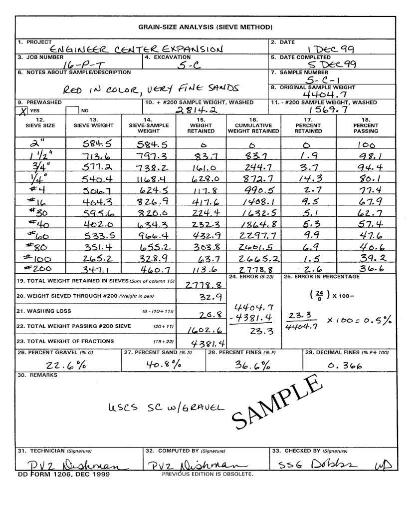
This is a sample sieve analysis result. For the lab (especially when sample washing is involved) it can get this complex, and the procedure is described in Materials Testing. To look at this more schematically (and this is common for most “textbook” problems) the following simplifications are done:

There are no losses in the process of sieve analysis. This is obviously unrealistic but these should be kept to a minimum. For textbook type problems this means that Blocks 8 and 23 are the same.
The tare (sieve or pan) weight is removed from consideration. This means that typically Column 15 is the first column in the problem, given the soil weights retained on each sieve. The weight that “hits the pan” is in Block 22.
Washing losses and errors are not considered, which means that Blocks 21 and 24 are set to zero.

With these out of the way, we can proceed to the analysis. The top sieve in the stack (the 2″ sieve) retained no soil (it doesn’t always happen this way) so it has zero soil retained and all passing. The next sieve (the 1 1/2″ sieve) retained 83.7 g (Column 15.) For the cumulative weight retained (Column 16) we add the value of Column 15 just above it to this one, thus 0 + 83.7 = 83.7 g. The next sieve (the 3/4″ sieve) retained 161 g, so for the cumulative weight retained for this sieve we add in the same way, thus 83.7 + 161 = 244.7 g. We keep going in the same way “down the stack” until we have all of the cumulative weights retained for each sieve computed.

This is terrific, but what we really need is the percentages of the total sample each cumulative retained value represents. This is what goes in Column 17. These values are obtained by dividing each result in Column 16 by the total sample weight in Block 23 and multiplying them by 100 to obtain a percentage. In this way, the cumulative percent retained for the 2″ sieve is obviously zero, for the 1 1/2″ sieve 83.7/4381.4 x 100 = 1.9%, for the 3/4″ sieve 244.7/4381.4 x 100 = 3.7%, and so on.

We can also compute the percent passing. An easy way to do this is to start by noting that 100% passes the whole sieve stack. We can than successively subtract the cumulative retained percentage as we go down. Thus the percentage of the 2″ sieve is again obviously 100 – 0 = 100%, for the 1 1/2″ sieve 100-1.9 = 98.1%, for the 3/4″ sieve 98.1-3.7 = 94.4% (note that we use the percentage passing from the previous sieve each time) and so on.

We then plot the results on the sieve curve as follows:

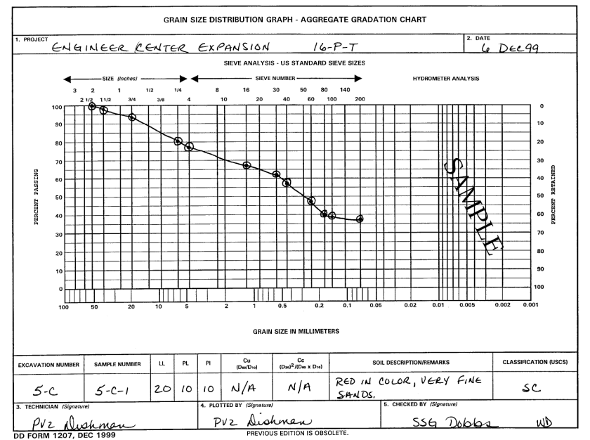
It’s a temptation these days to use a spreadsheet and its semi-logarithmic plotting features. I would avoid this: using a dedicated form like this has two advantages:

It lines up the grain sizes and sieve designations for you.
It can be plotted either from the percent passing size (left) or percent retained side (right.)

It’s also possible to use a tool such as the Spears Lab Spreadsheet, but this takes a lot of practice and is a little tricky to use, especially for “textbook” type problems where the tare is not considered. It’s easy to get a really stupid looking result; I have seen quite a few over the years.