Posted in Geotechnical Engineering, STADYN

A First Look at Estimating Beta Factors for Determining Pile Shaft Capacity of Driven Piles

In the last posting about STADYN, we put forth considerations for interface elements between the pile shaft and the soil.  Before we formally incorporate these into the model (or whether we will incorporate them or not) some consideration of how the interface actually works.  We will start those considerations by looking at methods by which the static capacity of driven piles is computed, and specifically the so-called “beta” methods which are used for cohesionless and sometimes cohesive soils.

Beta methods assume that the shaft resistance of the pile is a function of the effective stress of the soil along the pile shaft.  They assume that the horizontal stress that results from the vertical stress acts perpendicular to the surface of the pile.  The pile surface thus acts like a block on a surface with some kind of Coulombic friction acting against the downward settlement of the pile.  The beta coefficient is the ratio between the vertical effective stress and the horizontal friction on the pile, or

f_s = \beta \sigma'_o

\beta is in turn broken down into two components: the lateral earth pressure coefficient, which is the ratio between the horizontal and vertical stresses,

K = \frac {\sigma_h}{\sigma'_o}

and the coefficient of friction, or

\mu = tan \phi

We put these together to yield

\beta = K tan \phi

At this point let’s make two assumptions.  The first is that the lateral earth pressure coefficient is in fact the at-rest lateral earth pressure coefficient.  (For some discussion of this, you can view this slide presentation.)  The second is that the friction angle between the pile and the soil is in fact the same as the soil’s internal friction angle.  If we use Jaky’s formula for the at-rest condition, these assumptions yield

\beta = \left (1-\sin(\phi)\right )\tan\phi

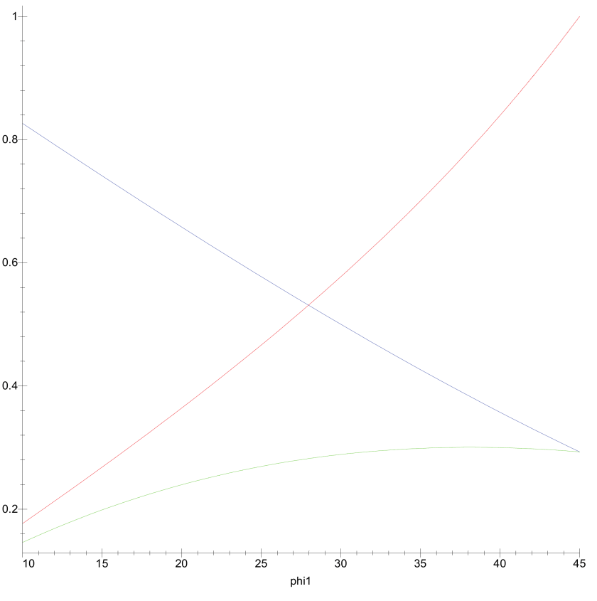
The various components of this equation are plotted below.
Beta Image 1

The three lines are as follows:

  • K_o = 1 - sin \phi is in red.
  • tan \phi is in blue.
  • \beta is in green.

It’s interesting to note that, as K_o increases, tan \phi decreases, and so \beta is within a surprisingly narrow range of values.  This plot is similar to one shown in Burland (1973), which we will discuss later.

If this were the case in practice, estimating \beta would be a straightforward proposition.  We’ll take two examples to show that this is not the case.

Let’s start with the Dennis and Olson Method for cohesionless soils, which is described here.  To arrive at \beta they do the following:

  1. They add a depth factor, which we will not consider.  Depth factors and critical lengths are common in static methods, but they are not well documented in the field.
  2. They assume K_o = 0.8 if their values for friction angle are used.
  3. They vary the friction angle from 15-35 degrees depending upon the type of soil.

Leaving out the depth factor, for this method \beta ranges from 0.21 to 0.56.  This is a considerably wider variation than is indicated above.  Since the depth factor is frequently greater than unity, this range is even larger.

An easier way to see this is to consider the method of Fellenius.  His values for \beta are as follows:

  • 0.15-0.35 for clay
  • 0.25-0.50 for silt
  • 0.30-0.90 for sand
  • 0.35-0.80 for gravel

Again the range of values is greater than the figure above would indicate.  Why is this?

Although it’s tempting to use a straight empirical approach, let’s back up and consider the structure of the basic equation about and the assumptions behind it.  There are several ways we can alter these equations in an attempt to match field conditions better by considering these assumptions and seeing what changes might be made.

The Two Friction Angles Aren’t the Same

The first one is suggested by the notation in Dennis and Olson: the internal friction angle of the soil and that of the soil-pile interface are not the same.  Retaining wall theory (when it considers friction) routinely makes this assumption; in fact, the ratio \frac {\delta}{\phi} routinely appears in calculations.  Let us rewrite the equation for \beta as

\beta = (1 - sin \phi) tan \delta

and be defining the ratio

m = \frac {\delta}{\phi}

we have

\beta = (1 - sin \phi) tan (m \phi)

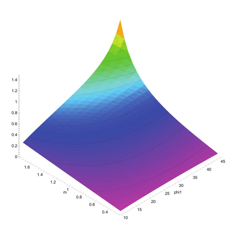
If we plot this in a three-dimensional way, we get the following result.
Beta Image 2.png

\beta is the vertical axis; m is varied from 0.25 to 1.75.  The results show that, for a given \phi , if we increase m we will increase \beta , and this increase is much more pronounced at higher values of \phi .

Although it’s certainly possible to have very high values of \delta = m \phi , as a practical matter in most cases m < 1.  Nordlund’s Method, for example indicates that m > 1 only with tapered piles, where a tapered pile face induces some compression in the soil in addition to shear.  In any case is m < 1 this will tend to depress values of \beta .  We should also note that using a ratio m does not mean that it will be a constant for any given soil.  This is especially true if \phi = 0 , where a multiplier is meaningless and we should have recourse to an additive term as well.

Jaky’s Equation Doesn’t Apply, or At-Rest Earth Pressure Conditions Are Not Present

Another assumption that can be challenged is that Jaky’s Equation doesn’t apply, or we don’t have at-rest earth pressure conditions.  Although Jaky’s Equation has done well, it is certainly not the last word on the subject, especially for overconsolidated soils (which we will discuss below.)  To try to “cover our bases” on this, let’s consider a range of lateral earth pressure coefficients by assuming that Jaky’s Equation is valid for the at-rest condition and that we need to somehow vary between some kind of active state and passive state.  The simplest way to do this is to assume Rankine’s conditions with level backfill, which just happens to be identical to Mohr-Coulomb relationships between confining and driving stresses.  (OK, it’s not all luck here…)  Thus,

K_a = \frac {1-sin\phi}{1+sin\phi}

and

K_p = \frac {1+sin\phi}{1-sin\phi}

Let us also define an active-passive factor called actpas, where actpas = -1 for the active state, 0 for the at-rest state and 1 for the passive state.  We then plot this equation

\beta = K(\phi,actpas) tan \phi

below.  Since we only have K values for three values of actpas, we’ll use a little Lagrangian interpolation in an attempt to achieve a smooth transition between the states.

Beta Image 3

We note from this the following:

  1. The dip in \beta for the high values of \phi and  -1 < actpas < 0 (states tending towards the active) may be more a function of the interpolation than the physics.  OTOH, if we look at NAVFAC DM 7.02, Chapter 3, Figure 1, we see a dip between the at-rest and active states for dense sands, which is what we would expect at higher values of \phi .
  2. Values of \beta for the active case show little variation.  Given that driven piles are subject to cavity expansion during installation, one would expect some passivity in earth pressures.  Drilled shafts are another story; however, if we look, for example, at O’Neill and Reese, values for \beta can certainly range higher than one sees with the active states above.  Bored piles, however, are beyond the scope of this discussion.
  3. For low values of \phi , there is little variation between the three states.
  4. If we compare these values with, say, those of Fellenius or Dennis and Olson, we cannot say that the fully passive state applies for most reasonable values of \phi , undrained or drained.  (Values in Nordlund, however, indicate higher values of K for larger displacements, approaching full passivity for large displacement piles.  Another look at this issue is here.)

Conclusion

If we compare the results we obtain above with empirical methods for determining \beta , we see that none of the variations shown above really allows us to match the theory we’ve presented with the empirical methods we’ve described (and others as well.)  As a general rule, \delta < \phi or m < 1 , so it’s safe to conclude that our assumption that the K can be determined using Jaky’s Equation only results in values of \beta that are too low.

It’s tempting to simply fall back on an empirical value for \beta , but for finite element analysis a more refined approach seems appropriate.  In subsequent posts we’ll look at such an approach, along with the issue of applying \beta methods to cohesive soils as well as cohesionless ones.

References

In addition to those in the original study, the following reference is mentioned here:

  • Burland, J.B. (1973) “Shaft friction of piles in clay – A simple fundamental approach.” Ground Engineering 6(3):30-42, January.

Posted in Academic Issues, Deep Foundations, Geotechnical Engineering

Tribute to Harry M. Coyle

It is with sadness that we report the death of Dr. Harry M. Coyle, professor of civil engineering at Texas A&M University from 1964 to 1987, back in January.  The obituary is below.

For those of us involved in deep foundations, his name is a familiar one, and his monographs have graced this site and its companion, vulcanhammer.info, for many years.  Among other things he is known for the Coyle and Castello method for estimating pile capacity in sand, the Coyle and Gibson method for determining damping for pile dynamics analysis, and the co-developer of the PX4C3 routine for axial load-settlement estimation, which we feature on this site, and which is the ancestor of many of those in use today.  He was deeply involved in the development of the TTI wave equation program, and some of his work relating to that is here.

Our continued condolences and prayers go to his family, and, as the obituary states, “Having loved his friends and family well, Harry Coyle will be missed by all until we are reunited with him in Glory. “

Obituary

Harry Michael Coyle, 90, entered the presence of his Savior on January 18, 2017. He was born on January 7, 1927 in Johnstown, PA to Foster H. and Ruth Enid Michael Coyle. Graduating from Richland Township, PA schools, Harry briefly enlisted in the Army, then won an appointment to the United States Military Academy at West Point, where he graduated in 1950. He earned a Masters Degree in Civil Engineering in 1956 from MIT and a PhD in 1963 from the University of Texas at Austin.

Harry met the love of his life, Josephine (Jo-Jo) Oefinger on a blind date in Washington, DC in 1954. It was love at first sight. Among other things, Harry told her, “Your eyes are like limpid pools and I could drown in them.” The star-struck couple married on March 26, 1955. Their love story lasted through 56 years of marriage at her death in 2011, and until this day.

Colonel Coyle actively served his country in the Army Corps of Engineers for 12 years: in Alaska after graduation from West Point; at Ft. Belvoir, VA (where his daughter, Debbie, was born in 1956); in a deployment to Korea in 1957 (during which daughter, Jenifer, was born in San Antonio); and on faculty at West Point (where son, Michael, was born in 1960). He then served as an officer in the U.S. Army Reserves while earning his PhD in Austin, where son, Pat, was born in 1963. Ultimately, he attained the rank of Colonel in 1973 and retired in 1987.

With his PhD in hand, Dr. Coyle took a job at Texas A&M University in the Civil Engineering Department in 1964, and moved the family to Bryan, Texas. A popular faculty member, he energetically served his Aggie colleagues and students until his retirement in 1987.

It was in the BCS community that Harry’s commitment and desire to serve his Lord blossomed. He and Jo-Jo became founding members of Grace Bible Church, where Harry served many years on the Board of Elders, eventually becoming an Elder Emeritus. For 50 years at Grace, he shared his deep faith and knowledge of the Bible with hundreds of students and many adults through small group teaching and one on one mentoring. Harry and Jo-Jo founded the Adopt An Aggie program at Grace, patterned after West Point’s adopt a plebe program. Known as a prayer warrior, Harry spent hours a day lifting up the needs of others, and he helped spread the Gospel of Christ throughout the world via financial and prayerful support of many missionaries. He continued to disciple, support and inspire others until his death. Having loved his friends and family well, Harry Coyle will be missed by all until we are reunited with him in Glory.

He was preceded in death by his parents, his beloved wife Jo-Jo, and his dear son Michael. Harry is survived by daughter Debbie Barry (and her children Julia and Andrew) of Belmont, MA; daughter Jenifer Purvis and husband Karl (and their children Kelsey and fiancée Scott Lorg, and Matthew and wife Morgan) of Berryton, KS; daughter-in-law Beth Gibson Coyle Faris of Boerne, TX and her daughters Christen (and husband Jacob) Kennington and Lauren (and husband Christopher) Orgeron of Houston, TX; son Patrick Coyle and wife Jeanne (and their children Katie, David and Lexie) of Bryan, TX ; and sister Lucretia Ann Cucciardo of Tampa, FL, and many loving nieces, nephews and cousins. Beloved great-grandchildren are Micah and Claire Orgeron, and Riley and Reagan Kennington.

A visitation will be held from 6:30 – 8:30 PM on Sunday, January 22, 2017 at Hillier Funeral Home of Bryan. A celebration of Harry’s life will be held at 11:30 a.m. on Monday, January 23, 2017 at Grace Bible Church, 700 Anderson Street, College Station. Memorial gifts may be given to Grace Bible Church Missionary House, 700 Anderson Street, College Station TX 77840; or Hospice Brazos Valley, 502 W. 26th St., Bryan, TX 77803.

Posted in Geotechnical Engineering, Soil Mechanics

Featured in Print: Materials Testing

Materials Testing CoverMost Soil Mechanics courses feature a lab course to go with them, either integral or separate.  The textbook manufacturers are quick to take advantage of that with expensive books and software.  ASTM specs are just about standard in the U.S., but trying to teach out of an ASTM spec is a trying business.

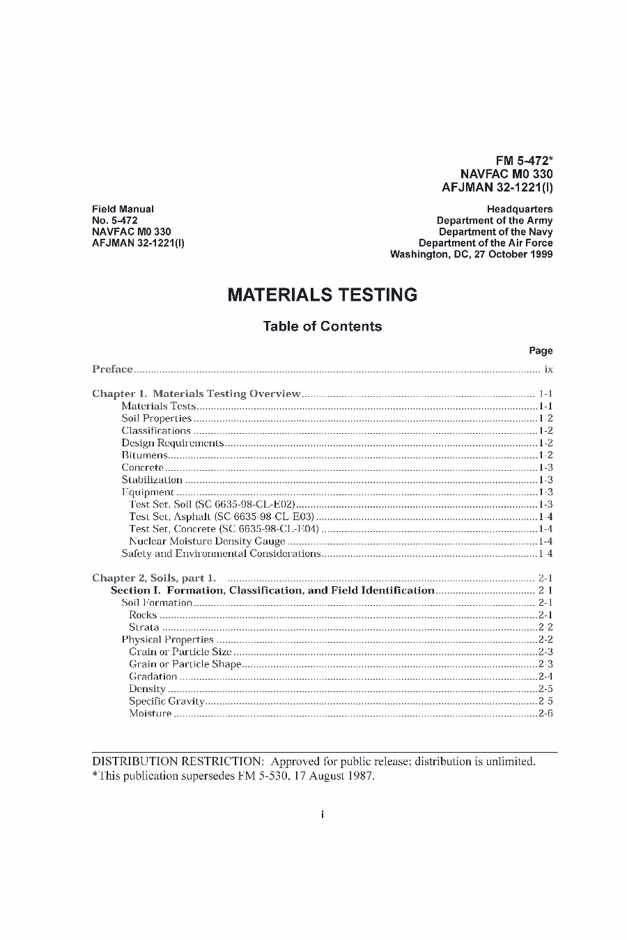
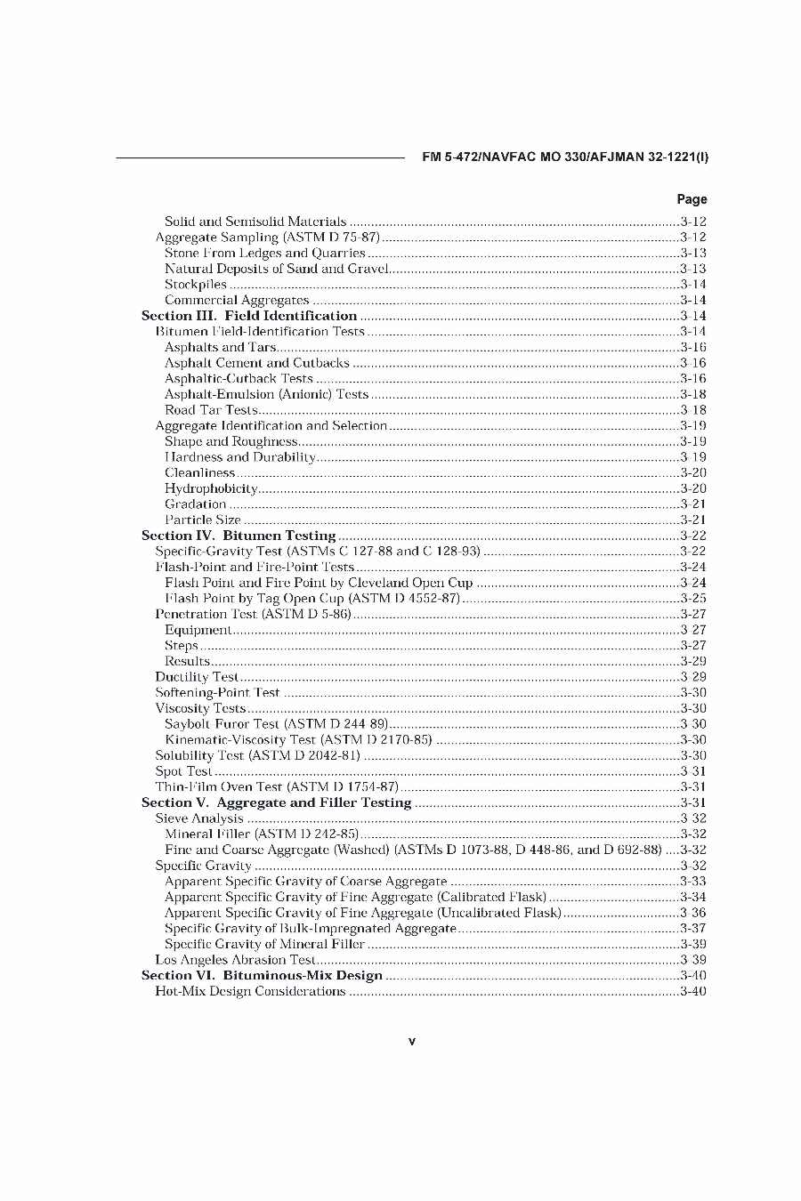
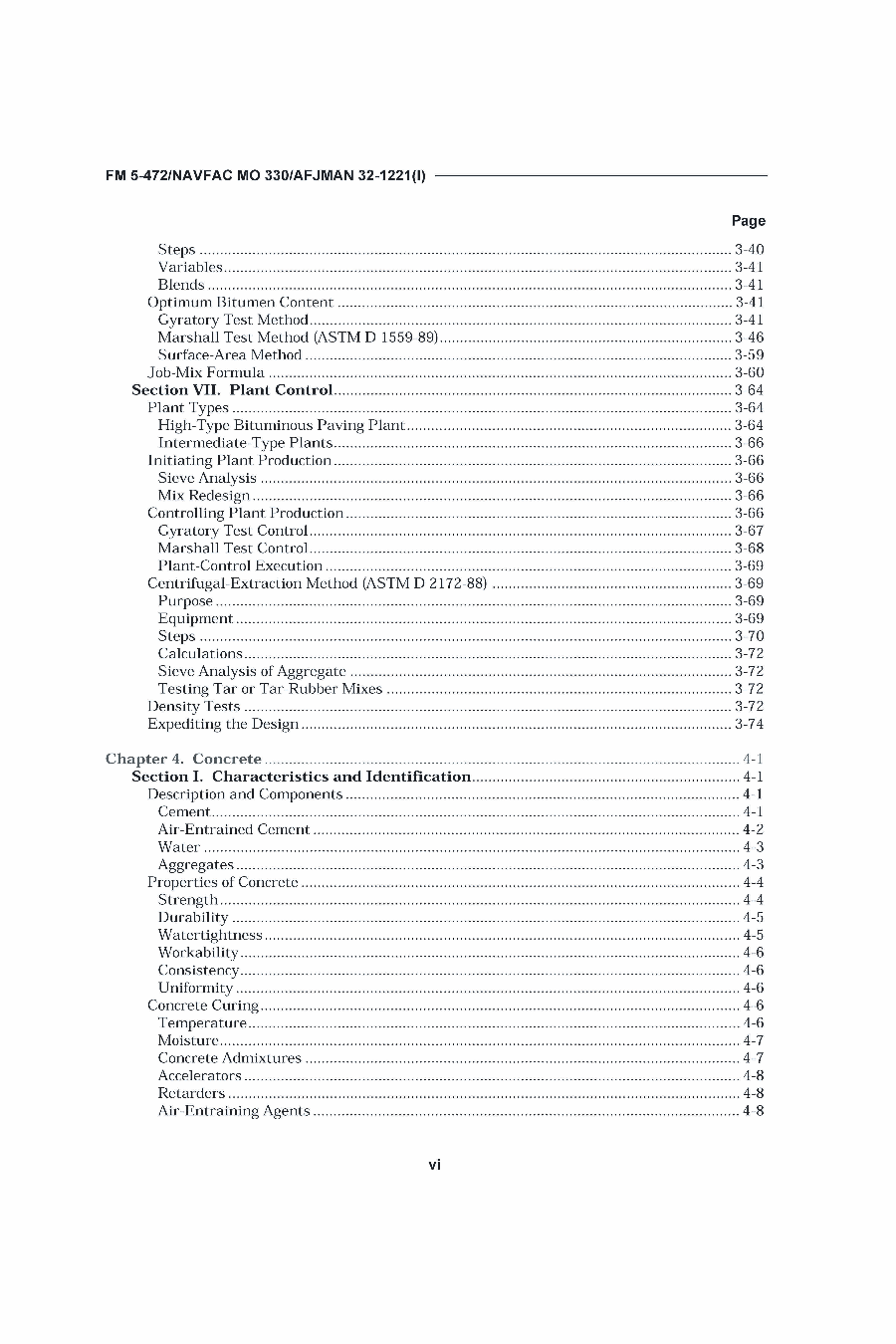
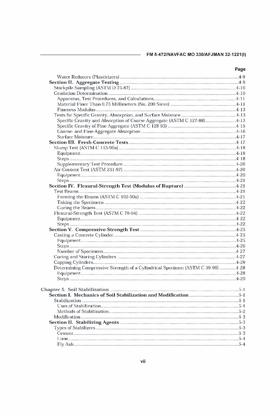
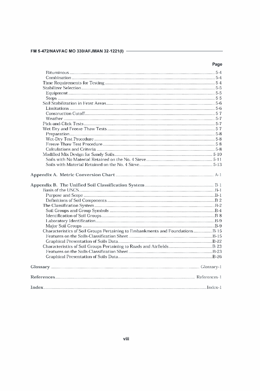
An alternative to this is Materials Testing, the print version of the U.S. Army’s FM 5-472.  In addition to the soils tests, it features many other items, some of which are not geotechnical tests at all:

  1. Materials Testing Overview
  2. Soils Testing
  3. Bituminous Mixtures Testing
  4. Concrete Testing
  5. Soil Stabilization

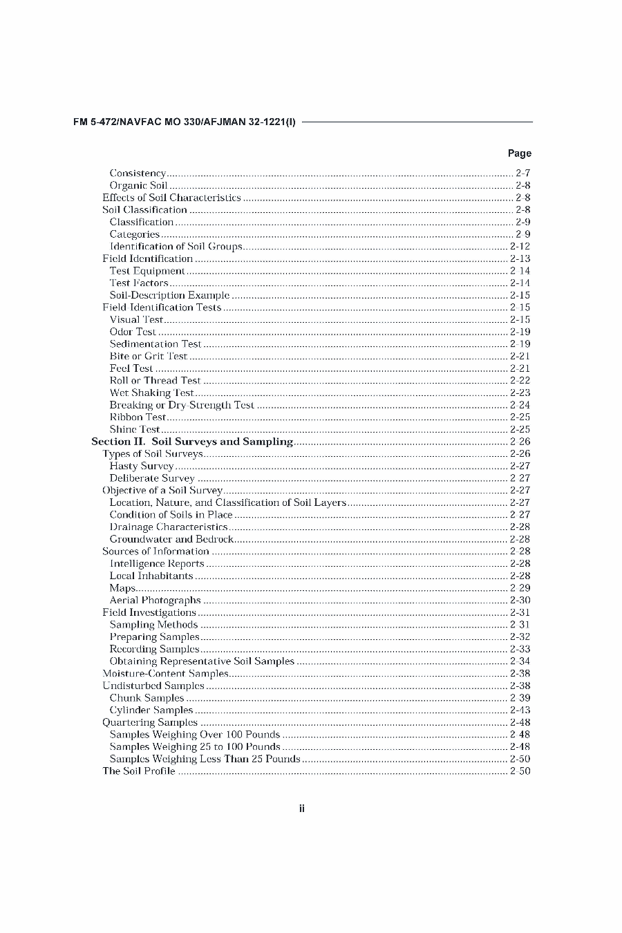
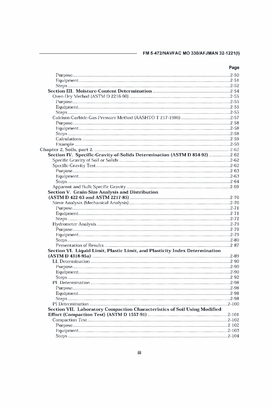
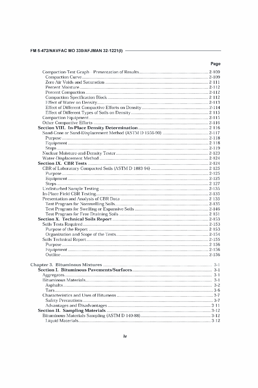
The soils tests in particular are as follows:

  • Moisture-Content Determination
  • Specific-Gravity-of-Solids Determination (ASTM D 854-92)
  • Grain-Size Analysis and Distribution (ASTM D 422-63 and ASTM 2217-85)
  • Liquid Limit, Plastic Limit, and Plasticity Index Determination (ASTM D 4318-95a)
  • Laboratory Compaction Characteristics of Soil Using Modified Effort (Compaction Test) (ASTM D 1557-91)
  • In-Place Density Determination
  • CBR Tests

You can view the table of contents below.

Pages from FM5-472_Page_1Pages from FM5-472_Page_2Pages from FM5-472_Page_3Pages from FM5-472_Page_4Pages from FM5-472_Page_5Pages from FM5-472_Page_6Pages from FM5-472_Page_7Pages from FM5-472_Page_8

Materials Testing is an excellent lab manual, supplementary textbook, or handy resource for the testing and improvement of soils, asphalt or concrete.