technology – vulcanhammer.net

Academic Issues, Geotechnical Engineering, Soil Mechanics

SLOPE Stability Software Program

Posted on 22 August 2026 by Don Warrington

Ever since this site’s predecessor was started in 1997, one of the things it’s “about” is offering useful documents and software at no charge. With software that’s become more difficult as operating systems have changed and some software has become inoperable on newer computer systems. We’ve gotten around that for DOS and Windows 3.1 applications, as shown in Partying Like It’s 1987: Running WEAP87 and SPILE (and other programs) on DOSBox. In this case we’re featuring a Windows-based, 32-bit software program for slope stability called–wait for it–SLOPE. It was developed by the late Arnold Verruijt, whose Soil Mechanics book I used for many years.

Downloading the Software

That’s pretty straightforward: click on the link below and save the file to your computer.

Download SLOPE Stability Software

What you’ll see is slope.zip. Computers and file download sites are getting nervous about raw Windows .exe files, so all you need to do is to extract the one and only slope.exe file from the archive.

Starting SLOPE

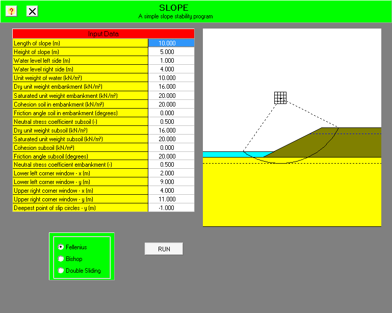
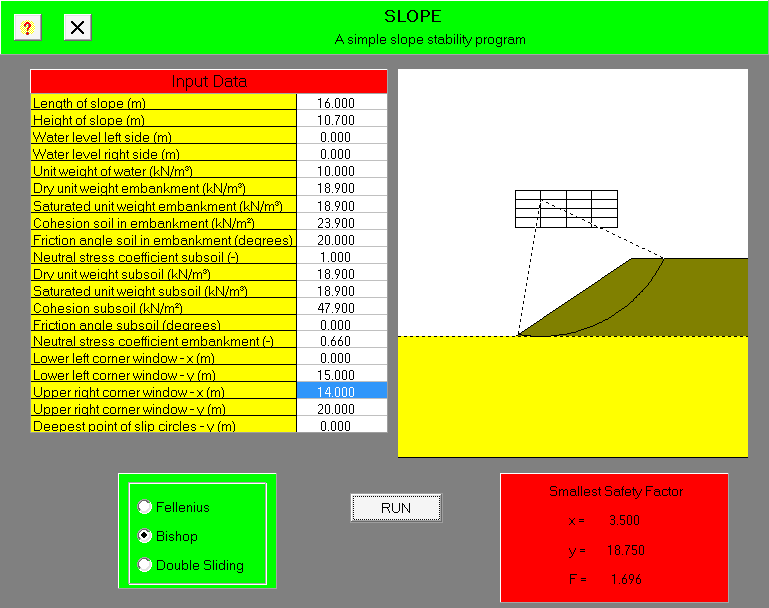
Now we come to the first discovery: slope.exe isn’t a program installation file, it is the program! You just double click on it and you will be greeted with the interface shown at the top of the post. The data entry is in the while column under “Input Data.” We will explain the input in an example.

The Example

The example is shown below, it is taken from the Soils and Foundations Reference Manual. The description from there is as follows:

Figure 6-20 shows a 35 ft high slope with a grade of 1.5H:1V. The soil properties within the slope and under it are shown on the figure. Groundwater is immediately under the slope. Calculate the factor of safety for a toe circle by using total stress analysis based on the soil properties shown.

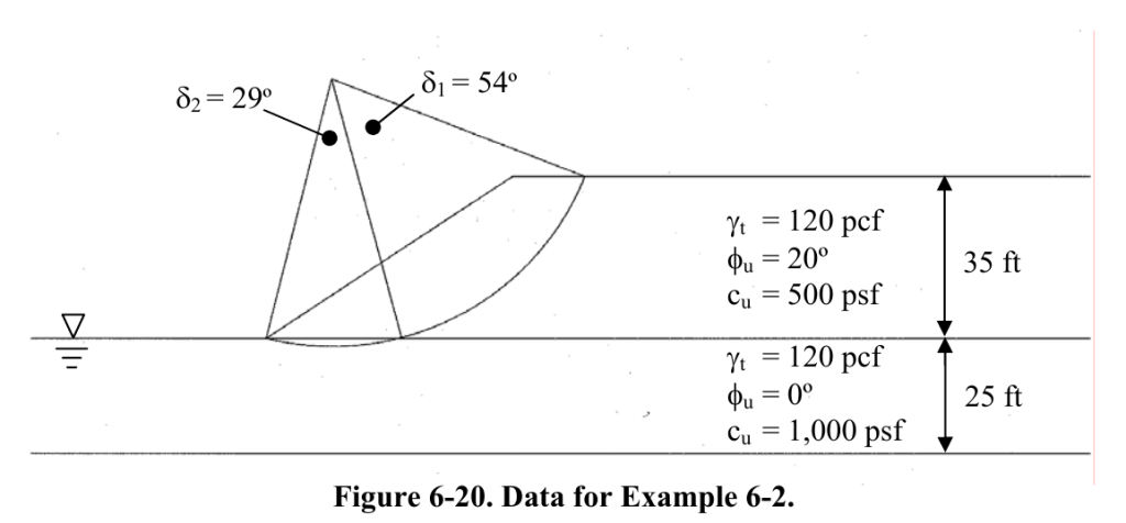
Because slope locates the slip circle of failure, we can ignore the geometry specified in that part of the drawing.

Basic Principle of Operation

SLOPE is based on classical slope stability techniques that goes back to Wolmar Fellenius’ work in the first part of the last century. It assumes that the soil fails along a circular surface, as shown below.

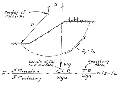
The weight of the soil is driving the soil downward, and this is resisted by the shear resistance along the failure surface (the dashed line.) That resistance is affected by a number of factors, including effective stress along the failure surface, friction of the particles, and cohesion of the soil. The whole mass rotates about the center of rotation, which has to be determined during analysis.

The most common method used–and the one SLOPE uses–is the method of slices. In that method the soil mass is divided into vertical slices, each of which has a mass, some kind of resistance along the failure surface, and (for most of the methods used) how the slices interact with each other.

The theory is described in both Soil Mechanics and the Soils and Foundations Reference Manual. The computations can be laborious, but the really tricky part is determining the location of the center of rotation and the radius R of the failure surface. SLOPE takes care of all of that but it is essential for you to understand how it does that, as its determination of all of these factors is not automatic.

Dealing With Different Expressions of Slope

One common problem with slope stability situations is how the geometry of the slope is defined. There is more than one way of doing it, and the method used in the problem is different than the one used in SLOPE.

The problem states that the slope is 35′ high (the vertical length of the slope) with a grade of 1.5H/1V. This means that, for every foot or meter of height, there are 1.5 feet or meters of horizontal length. In this case the horizontal length is (35)(1.5)/(1) = 52.5′. Alternatively we can compute the angle of slope as arctan(1/1.5) = 33.7 degrees, in which case the length is 35/tan(33.7) = 52.5′

Inputting the Data

SLOPE requires the data to be put in SI units. We will do the conversions as we proceed. The data input is as follows:

Length of slope (m) = 52.5′ = 16 m
Height of slope (m) = 35′ = 10.7 m
Water level left side (m) = 0 (from problem statement, zero is at the toe of the slope)
Water level right side (m) = 0 (again from problem statement)
Unit weight of water (kN/m³) = 10 (reasonable approximation)
Dry unit weight of embankment* (kN/m³) = 120 pcf = 18.9 kN/m³
Saturated unit weight of embankment (kN/m³) = 18.9 (in absence of better data, use the same)
Cohesion soil in embankment (kN/m²) = 500 pcf = 23.9 kN/m²
Friction angle in embankment (degrees) = 20 (from problem statement)
Neutral stress coefficient subsoil** = 1.00
Dry unit weight subsoil* (kN/m³) = 120 pcf = 18.9 kN/m³
Saturated unit weight subsoil (kN/m³) = 18.9 (in absence of better data, use the same)
Cohesion soil subsoil (kN/m²) = 1,000 pcf = 47.9 kN/m²
Friction angle subsoil (degrees) = 0 (from problem statement)
Neutral stress coefficient embankment** = 0.66
Lower left corner window*** – x(m)
Lower left corner window*** – y(m)
Upper right corner window*** – x(m)
Upper right corner window*** – y(m)
Deepest point of slip circles – y(m) = -25′ = -7.6 m (this is negative as it is below the toe of the slope)

Notes:
* The embankment is above the toe. The subsoil is below it.
** The neutral stress coefficient is more commonly referred to in American practice as the at-rest earth pressure coefficients. For normally consolidated soils, it equals to $1 - \sin(\phi)$ , and the results are shown in the input list. The entry points for both are out of order, so be careful.
*** This will be explained below.

Choosing the Window Points and the Method of Analyzing the Slices

If we put all of this data into SLOPE, we get the following result:

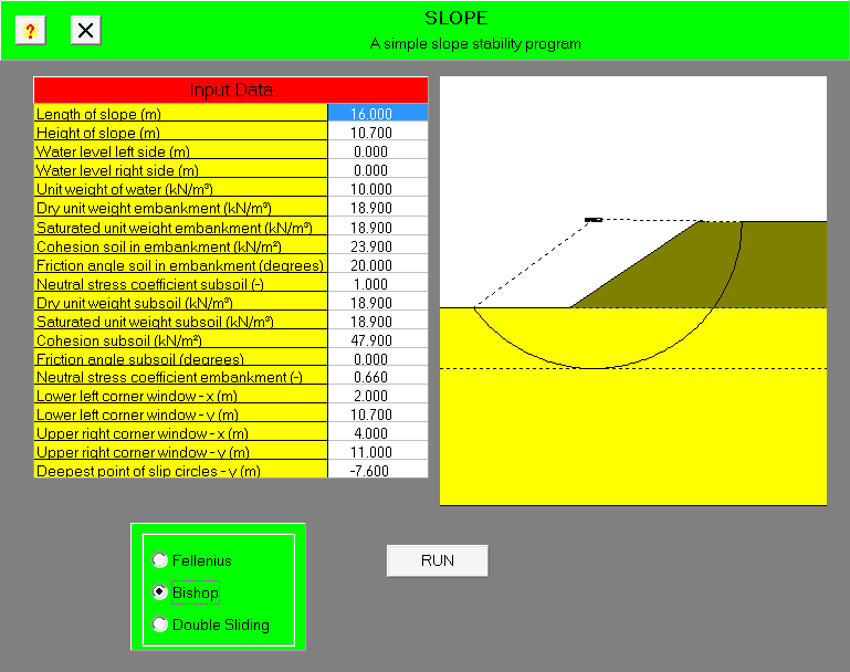
Before we get some results, we have to make two decisions: what slice analysis method to use and the extent of the window.

Soil Mechanics gives an explanation of Fellenius and Bishop’s methods. SLOPE divides the region in the slip circle into the horizontal slices; the difference between these two methods is that Fellenius’ method does not consider friction between the slices while Bishop’s does. Fellenius’ method does not require an iterative solution and is the most conservative; however, given that the computational effort is done by the program, we will use Bishop’s method, which is in common use.

As far as the “window” is concerned, SLOPE, in common with many slope stability programs, uses a grid optimization method to find the location of the rotational centre. This means that a set of points in a regular grid are each analyzed (along with appropriate slip circles) to get the factor of safety (see sketch above) and after analyzing all of these points picks the one with the lowest factor of safety. It’s easy to see that, using the original grid, not much in the way of useful information can be found as the selection of grid points is too small. For a grid point to be valid, it has to be in the interior of the window, not at the edge, because if it’s at the edge it’s possible that the point will be outside of the window.

The window limits are set using a coordinate system with the origin at the toe of the slope. Generally the slip circle centre will be above and to the left of the upper corner of the slope. Values for y should not be less than the slope height and values for x should be greater than zero and less than the length of the slope.

Getting an acceptable result is an iterative process. Let us assume the following for the window boundaries:

Lower left corner window*** – x(m) = 2 m
Lower left corner window*** – y(m) – 10.7 m
Upper right corner window*** – x(m) – 14 m
Upper right corner window*** – y(m) – 15 m

If we apply these and then Bishop’s method for the analysis, we get the following result:

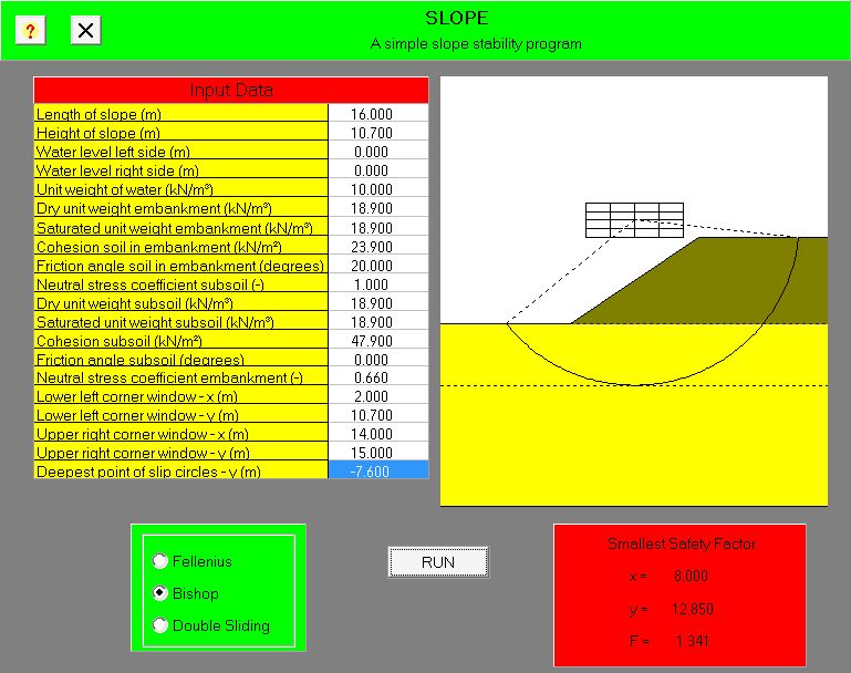
We can see the slip circle centre is in the interior of the grid. If we desire we can shrink the window to get a finer grid and a more precise result.

Sometimes assuming the slip circle going to its lowest point does not result in the lowest factor of safety. To simulate something close to a toe circle, let us set the deepest point at the bottom of the embankment; the result we obtain is as follows:

In this case (with some adjustments to the window) the factor of safety is still higher for our original case.

Reporting the Results

SLOPE is not installed, and as a result does not print out its results. The only way to save the results from the program is to get them off of the screen. This is fairly straightforward: use a grab or screenshot program, which was done with the images in this post. Unfortunately many of my students, for whatever reason, insisted on using their phones to take shots of the literal screen, which generally look awful. This was the technology I used forty years ago when presenting this program; we’ve come a long way since.

Conclusion

SLOPE is a fairly simple program to use. It lacks many of the automation and stratigraphy defining features other slope stability software packages have, and is not suited for use in practice. For academic use, however, it is good, and gets students past one of the most tedious features of geotechnical computation.

Uncategorized

Net vs. Gross Ultimate Bearing Pressure

Posted on 18 August 202618 August 2026 by Don Warrington

When you’ve taught any course for as long as I taught Soil Mechanics and Foundation Design and Analysis, you’ll sometimes get inquiries from your students about topics that you either didn’t cover or they might have missed. (Many comforted themselves during the course with the thought that “I’ll never go into geotech,” only to have it be their first job.) This topic came from a student from Florida (which is, of course of special interest for a long list of reasons, esp. since I grew up there) who saw on a geotech report about bearing pressure on a shallow foundation (in this case, a pool) citing the net bearing pressure on the foundation.

The topic applies to both bearing capacity and settlement of shallow foundations. The simplest illustration of this I could find is at the top of the post; it comes from the presentation of Schmertmann’s Method of settlement estimation from the Soils and Foundations Reference Manual, and I discussed it in Foundation Design and Analysis: Shallow Foundations, Settlement.

Using the notation above, the pressure p is the gross bearing pressure on the foundation. The pressure p₀ is the effective stress at the base of the foundation. The difference between the two is Δp, which is the net bearing pressure on the foundation.

So how is this relevant to foundation design? In the case of Schmertmann’s Method, it is a part of the method. For bearing capacity, the Soils and Foundations Reference Manual has the following to say:

The net ultimate bearing pressure is the difference between the gross ultimate bearing pressure and the pressure that existed due to the ground surcharge at the bearing depth before the footing was constructed, q (= γ_aD_f). The net ultimate bearing pressure can thus be computed by subtracting the ground surcharge (q) from Equation 8-6:

q_{ult net} = q_ult – q (8-14)

q_{ult net} = cN_cs_cb_c + q (N_q−1) C_wq s_qb_qd_q + 0.5γB_fN_γC_wγs_γb_γ (8-15)

The structural designer will typically include the self-weight of the concrete footing and the backfill over the footing (approximately equal to γ_aD_f) in the loads that contribute to the applied bearing stress. Therefore, if the geotechnical engineer computes and reports a net ultimate bearing pressure, the effect of the surcharge directly over the footing area is counted twice. Reporting an allowable bearing capacity computed from a net ultimate bearing pressure is conservative and generally not recommended provided that a suitable factor of safety is maintained against bearing capacity failure. If the geotechnical engineer chooses to report an allowable bearing capacity computed from a net ultimate bearing pressure, this fact should be clearly stated in the foundation report.

Bearing capacity theory is explained in Chapter 11 of Soils in Construction.

In general, the ultimate capacity is the more conservative option to use. Combined with the difficulties associated with bearing capacity analysis, I decided not to emphasise net bearing capacity in my teaching. Additionally, for a small pool like the one we had in Palm Beach, bearing capacity failure is remotely possible. For a large (say, Olympic) size pool, we’re dealing with something approaching a mat foundation, and these generally fail in settlement, as noted in Foundation Design and Analysis: Shallow Foundations, Other Topics.

Geotechnical Engineering, Soil Mechanics

Once More With Feeling on Hough’s Method

Posted on 19 June 2025 by Don Warrington

I recently received in inquiry from an organisation which has proposed a shallow foundation of an embankment. They used (wisely IMHO) an FEA analysis to estimate the settlement. The owner’s response was that, since their result was a little greater than Hough’s Method, and Hough’s method reputedly overestimates the settlements by a factor of 2, that the FEA analysis overestimated the settlements. They referred this person to my posts Getting to the Legacy of B.K. Hough and his Settlement Method and Closing the Loop (or at least trying to) on Hough’s Settlement Method, which is evidently about the only ongoing discussion of the topic around these days.

Both of these posts have two objectives: a) they attempt to trace the development of the method, both by Hough and those who came after, and b) to begin the journey to a resolution of the accuracy of the method. The problem with both of these is that the problem is simple to state but, because of the nature of the evidence, difficult to resolve. I’ll start with a brief review of these two objectives and then set forth a worked example (something that is admittedly lacking in my first two posts) to see how things work out. I’ll end with some thoughts on how to more accurately determine the values of C’, which is the core issue with this method.

The Method and Its Development: A Review

“The SPT is a dynamic test, while soil bearing capacity is a matter of statics, interpreting one in terms of the other is analogous to determining the bearing capacity of piles from pile driving formulas. Consequently, it is felt that attempts to present correlations between blow counts and bearing capacities of soils would be an oversimplification of a much too complex subject.” From Fletcher (1965)

“Hough’s Method” is not univocal; he presented it in two forms in Hough (1959) and Hough (1969). The governing equation is the same for both:

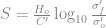
$S=\frac{H_{o}}{C'} \log_{10} \frac{\sigma'_f}{\sigma'_o}$ (1)

This equation is identical to Equation (3) of my post The Sorry State of Compression Coefficients except for the form of the variables. In some places equations like this are used for fine-grained soils; this is explained in Verruijt.

The basic problem is determining C’ and there are two difficulties with this:

Hough changed the SPT N vs. C’ curves in the intervening decade between the two forms.
We’re not informed what type of SPT hammer Hough used, or if/how he corrected them as we do now (there’s no evidence that he did.)

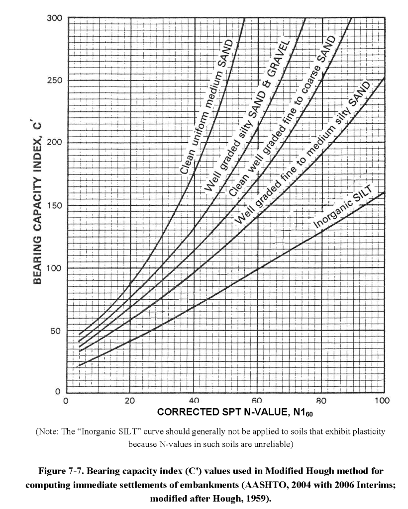
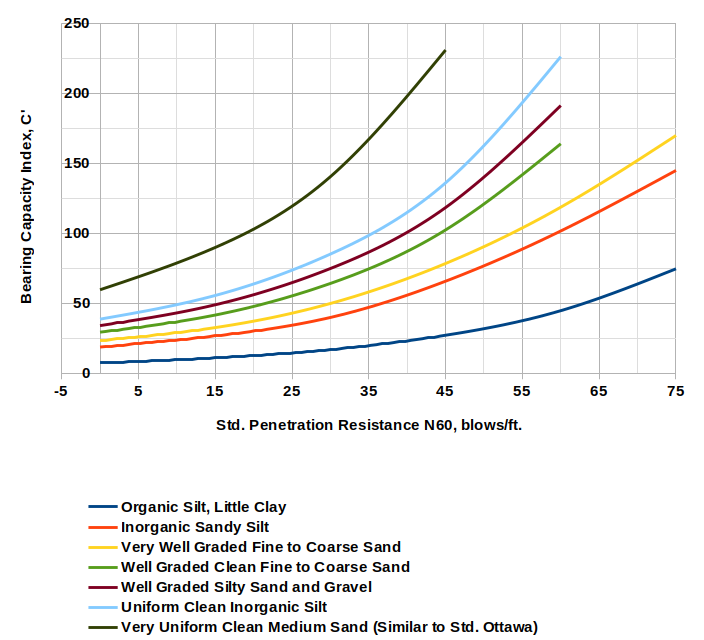
Let’s start with the first problem: the curves reproduced from the 1959 version (from the FHWA’s Soils and Foundations Manual) are here:

Figure 1 Bearing capacity index (C’) values used in Modified Hough method for computing immediate settlements of embankments (from FHWA (2006))

We’ll deal with the business of N1₆₀ shortly. There is no evidence that Hough meant to restrict his method to embankments.

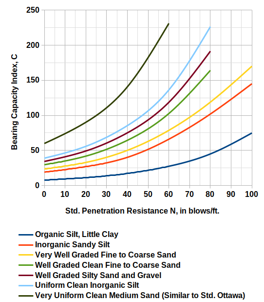
The chart from the 1969 version is reproduced below (my reproduction):

Figure 2 Hough’s Method Relationship between N Values and C’ Values (redrawn from Hough (1969))

One of the more thoughtless things the FHWA has done in publishing this method is never presenting any equations for these curves, which are easily obtained using linear regression. I have done this and you can see them in Getting to the Legacy of B.K. Hough and his Settlement Method.

Obviously these sets of curves are not identical; the soil classifications he uses aren’t either, and there are five (5) curves in the 1959 version while there are seven (7) in the 1969 one.

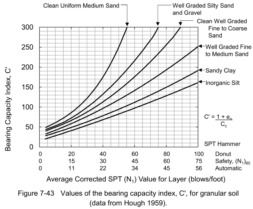
Turning to the second problem, in neither of Hough’s original monographs is any kind of correction–mechanical or overburden–are mentioned. The FHWA has consistently added overburden correction. As far as mechanical correction is concerned, in Design and Construction of Driven Pile Foundations, 2016 Edition the FHWA has assumed (not unreasonably) that Hough obtained data from a donut hammer and their correction (which also includes overburden correction) looks like this:

Figure 3 Values of the Compression Index C’ for granular soil (from FHWA (2016))

In the same vein I shifted the x-axis of Figure 2 for N₆₀ values as shown below.

Figure 4 Relationship of N₆₀ Values to C’ for Hough (1969) Method Assuming Original Donut Hammer

Equations for these curves are included in Closing the Loop (or at least trying to) on Hough’s Settlement Method.

A Worked Example

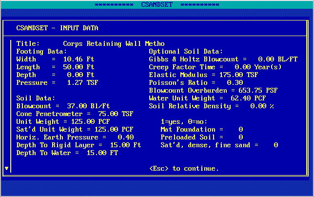
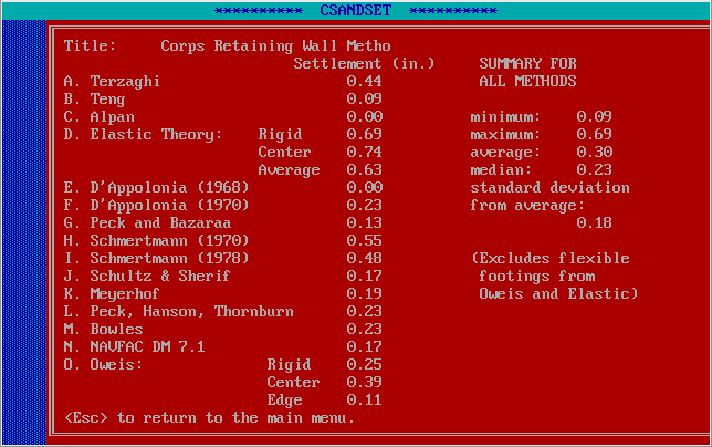
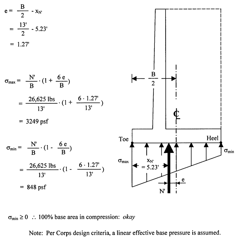
With that out of the way, the best way to illustrate the use of Hough’s Method is using a worked example, in this case a retaining wall foundation from A Simplified Method to Design Cantilever Gravity Walls. The diagram at the top of the page shows the foundation; the settlement calculations for a variety of methods (using the U.S. Army Corps of Engineers’ CSANDSET program) are given there. Let’s begin by reproducing those results below.

This program includes a fairly broad selection of methods, from elastic/theoretical ones to purely empirical ones. These methods are described in the program manual. While some of them may not be really applicable to this type of foundation, they show the wide variations of these methods, which suggests that there is not a consensus on computing these values.

Hough’s Method is not included. The detailed solution to the problem is contained in this spreadsheet. We assumed that the soil was well-graded fine to medium sand. There are four variations to the results, which are shown below:

Variation on Hough’s Method	FHWA SFH Method	FHWA DPF Method	Closing the Loop (or at least trying to) on Hough’s Settlement Method proposal, no overburden correction	Closing the Loop (or at least trying to) on Hough’s Settlement Method proposal with N1₍₆₀₎ Values
Settlement, in.	0.647	0.466	1.162	0.553

As has been documented widely, the results of Hough’s Method are generally above most of the methods used in CSANDSET, although in the case of Schmertmann’s Method (which has been widely disseminated) the difference is not so great. The largest of the Hough’s Method variations is the Closing the Loop (or at least trying to) on Hough’s Settlement Method proposal, so I ran this with the N1₍₆₀₎ values, which resulted in settlements between the two FHWA methods.

One thing I would caution about using an “academic” problem as an illustration is that the parameters–many of which are taken from “typical” values–may not be representative of what actually occurs in the field, and may yield less than satisfactory results, especially for methods with a strong empirical basis. I ran into this problem with Driven Pile Design: Three Methods of Analysis. On the other hand field results are specific to their location and may not be representative of soils that the geotechnical engineer can expect to encounter.

New Values of C’

I’m not sure how much progress has been really made in this discussion. First I summarised my last two posts on Hough’s Method and how it comes up with the value of the compression constant C’, which is an alternative method of using consolidation settlement techniques to estimate one-dimensional settlement. Then I applied this to an example. Both of these have some value but they don’t get to the heart of the issue: we need more reliable (or at least values of which we understand the source) of the compression constant C’.

One hallmark of many of the fixes for this method is the invocation of overburden correction, which (as we saw above) reduces the resulting settlement. Doing this reminds me of something my Computational Fluid Dynamics I professor put in his notes many years ago:

Also, a few words need to be said about how one should interpret results ensuing from a computational simulation. There are a couple of anecdotal-based observations that are often used to describe how to approach a calculated result: (1) Computed results are guilty until proven innocent, and (2) There’s nothing more dangerous than answers that look about right. These observations are related but have slightly different interpretations. The first says that newly computed results should always be viewed with aggressive skepticism. In other words, a CFD practitioner should never accept a computed result as “truth” or representative of Mother Nature until exhaustive means have been taken to ensure that the result is a “reasonable” approximation to reality. The second observation simply means that if a calculation gives results that are orders of magnitude different from those intuitively expected, then the results can usually be quickly judged as erroneous and there is work to do to find out why. The difficult part comes when a calculation gives results that are “close” to what was expected. Such an outcome often lulls the researcher and/or practitioner into thinking that “all is well” and there is no reason to continue scrutinizing the results. However, it is very possible that a “good” answer was obtained for the wrong reason.

Compression constant typical values aren’t exactly plentiful. This table, from Verruijt, is one I have put in my course materials for many years (for log₁₀ formulations):

Type of Soil	C’
Sand	20-200
Silt	10-50
Clay	4-40
Peat	1-10

Another tabulation comes from this source, converted to log₁₀ values:

Soil	Minimum C’	Maximum C’
Loess silt	6.5	19.6
Clay	13.0	52.2
Silts	26.1	65.2
Medium dense and dense sands	65.2	87.0
Sand with gravel	108.7	None

Hough (1969) himself suggests another way forward. Referring to his table of compression coefficient parameters reproduced in Getting to the Legacy of B.K. Hough and his Settlement Method, we start by noting that he computes the values of Cc using the following equation:

${\it C_c}=a\left ({\it e_0}-b\right )$ (2)

Since the compression coefficient and constant are related in this way

${C'}^{-1}={\frac {{\it C_c}}{1+{\it e_0}}}$ (3)

we can combine these equations and compute the compression constant thus

$C={\frac {{1+\it e_0}}{a\left ({\it e_0}-b\right )}}$ (4)

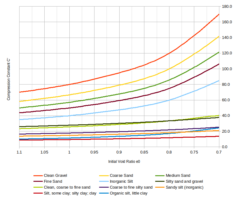
Doing this for Hough’s values of a and b (and one should be aware of the caveats he puts on values of b) for a range of void ratios yields the following tabular result:

	Hough’s Coefficients		Initial Void Ratio e₀ (first row) Values of C’ (rows that follow)
Soil Type	a	b	1.1	1	0.9	0.8	0.7
Clean Gravel	0.05	0.5	70.0	80.0	95.0	120.0	170.0
Coarse Sand	0.06	0.5	58.3	66.7	79.2	100.0	141.7
Medium Sand	0.07	0.5	50.0	57.1	67.9	85.7	121.4
Fine Sand	0.08	0.5	43.8	50.0	59.4	75.0	106.3
Inorganic Silt	0.1	0.5	35.0	40.0	47.5	60.0	85.0
Silty sand and gravel	0.09	0.2	25.9	27.8	30.2	33.3	37.8
Clean, coarse to fine sand	0.12	0.35	23.3	25.6	28.8	33.3	40.5
Coarse to fine silty sand	0.15	0.25	16.5	17.8	19.5	21.8	25.2
Sandy silt (inorganic)	0.18	0.25	13.7	14.8	16.2	18.2	21.0
Silt, some clay; silty clay; clay	0.29	0.27	8.7	9.4	10.4	11.7	13.6
Organic silt, little clay	0.35	0.5	10.0	11.4	13.6	17.1	24.3

Graphically this is what it looks like:

Although I would be reluctant to reconstruct the method based on this, it shows one important thing: there’s more than one way to get to these constants. If we want to have a method for consolidation settlement type solutions for cohesionless soils, we need to pursue all of the following:

SPT correlations, based on current practice for correcting and applying the results.
CPT correlations. Although not appropriate in all stratigraphies (what method is?) CPT is very useful and more consistent than the SPT in those stratigraphies where it can be applied successfully.
Basic soil properties such as void ratio, relative density and unit weight. This suggests lab tests on undisturbed samples; the problem here is that getting undisturbed samples of cohesionless materials into a consolidation testing machine is easier said than done.

It’s also possible to use tests such as the pressuremeter and dilatometer, but these would only be meaningful in places where they are commonly used.

Doing all of these things would advance our understanding of the settlement of shallow foundations and give us more meaningful comparison with finite element methods.

Unlinked References

Fletcher, G.F.A. (1965) “Standard Penetration Test: Its Uses and Abuses.” Journal of the Soil Mechanics and Foundations Division : Proceedings of the American Society of Civil Engineers. Vol. 94 No. 4, pp. 67-75. It is interesting to note that Fletcher cites Hough’s First Edition of Basic Soils Engineering, while Hough (1969) cites Fletcher (1965).
Hough, B.K. (1959). “Compressibilty as the Basis for Soil Bearing Value,” Journal of the Soil Mechanics and Foundations Division, ASCE, Vol. 85, Part 2.
Hough, B.K. (1969). Basic Soils Engineering. Second Edition. New York: Ronald Press Company.

Uncategorized

NAVFAC DM 7.2: Earthwork, Hydraulic and Underwater

Posted on 17 April 2025 by Don Warrington

The whole topic of earthwork and compaction is one whose coverage is inconsistent, to say the least, in basic geotechnical publications. Some do a very good job, others ignore it altogether. NAVFAC DM 7.2 has done a very thorough job on the subject, covering topics which are scarce in other places. Compaction is the oldest earth improvement technique we have and is still the most commonly used on construction sites around the world.

There are many topics which are explored in this chapter; I will only mention a few of them. It’s hard to distill all of the information in the book; you’ll just have to get it and find out for yourself. Some of them (such as compaction equipment types and sample fill specifications) are carried over and expanded from the previous document; others are new.

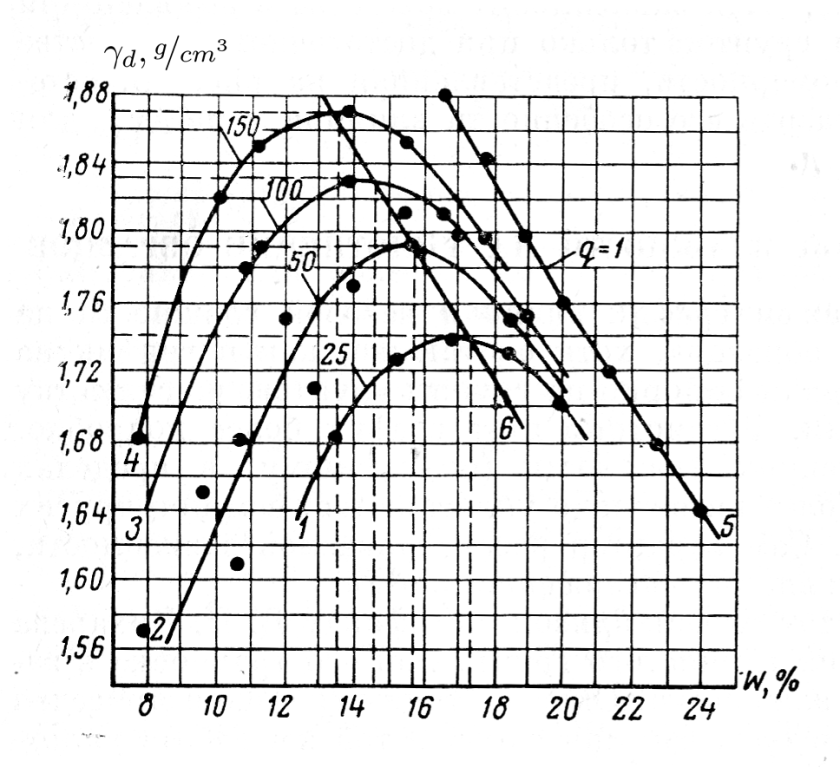
Line of Optimums Method

When I was first brought on board to Soils in Construction, I learned about this, which I discuss in this post (illustration of the method is at the right.) There were few references on the subject to be found, which made Soils in Construction somewhat unique. (I need to say kudos to my co-author, Lee Schroeder, especially for the part of the book on compaction.) We actually got thumbs up during the review process for including it. This edition of NAVFAC DM 7.2 has fixed that lacuna with a section on the subject. I don’t see how one can actually specify a compaction method without it, especially if experience is lacking and/or the soils are variable on a site. They have included information on the effects of “dry of optimum” (left of line 6 on the chart above) and “wet of optimum (right of line 6) as well. All in all, a very nice treatment on the subject.

Making the Cut with Borrow and Fill Calculations

Another topic covered in Soils in Construction is that of borrow and fill calculations. Some soil mechanics books cover this, some don’t. It’s covered in detail in NAVFAC DM 7.2. It will definitely help you to “make the cut” when excavating, transporting, placing and compacting fill materials.

Hydraulic Fills

Many geotechical references treat hydraulic fills as a thing of the past after some early disasters involving them. Evidently not; there is a whole chapter on the subject, both for understanding dams built in this way and for underwater fills, when hydraulic fills are virtually unavoidable.

Geotechnical Engineering

It’s Important to Have Enough Soil Borings on a Jobsite

Posted on 10 December 2024 by Don Warrington

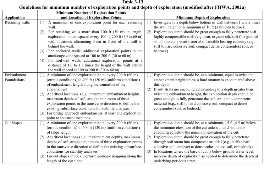
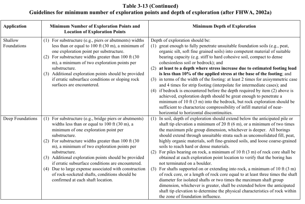
One thing that irritates me to no end is to look at a set of geotechnical plans and to realise that there is only one boring for the entire site. In a few cases that’s enough, but very few. The “uniform site conditions” of academic legend are seldom found in real life; soil conditions vary from one place to another on a site and in some stratigraphies in a matter of feet or metres. If it’s worth sending a crew out to a site for one or two borings it’s worth getting more.

The table “Guidelines for minimum number of exploration points and depth of exploration” is shown below, and is taken from the Soils and Foundations Reference Manual, which has much additional information on this and other related topics. It also deals with another issue that bedevils geotechnical exploration: going deep enough to get the information needed, especially with deep foundations. I also spent a great deal of time on this subject in my course Foundation Design and Analysis: Boring Logs and Their Interpretation, evidently more than other undergraduate courses.