One item that has become a staple in my Soil Mechanics course is this video, produced at the University of California at Davis about twenty years ago and revised in 2012.
It’s a lot easier to explain this topic with this video than through a book or long lecture.
Geotechnical specialty engineering and construction contractor Nicholson Construction is pleased to announce the addition of industry expert Mary Ellen Large, P.E, D.GE to the team. Ms. Large will be assuming the role of Client Care […]
Until recently she was Technical Activities Director for the Deep Foundations Institute, a fact which takes some digging to ascertain on their website.
In our last post on the subject we discussed the concept of resultants as replacements for simplicity of calculations. We’ll expand on the topic here by discussing two examples: surcharge retaining loads and loads on shallow foundations.
Obviously condensing that kind of distributed load into a resultant requires more serious integration that you have for a uniform or triangular load. In the past using a resultant was common in hand solutions of sheet pile problems; with software, if it has the option for something other than uniform surcharge (SPW2006 for example does not) it generally reproduces the distributed load.
One other use of a resultant concerns strip vs. line loads. You’ll notice that the information for line loads is more extensive than strip loads. One reason is that engineers commonly convert a strip (distributed) load into a line (resultant) load by multiplying the width of the load by its pressure and placing the load in the middle of the strip (assuming, of course, the distributed load is uniform.)
Shallow Foundations
Shallow foundations offer an interesting situation because in some ways we reverse the process, starting with a resultant and end up with a distributed load. We’ll restrict the discussion to the simplest case, a continuous foundation, in this case under a gravity retaining wall. Other cases are discussed in more detail here.
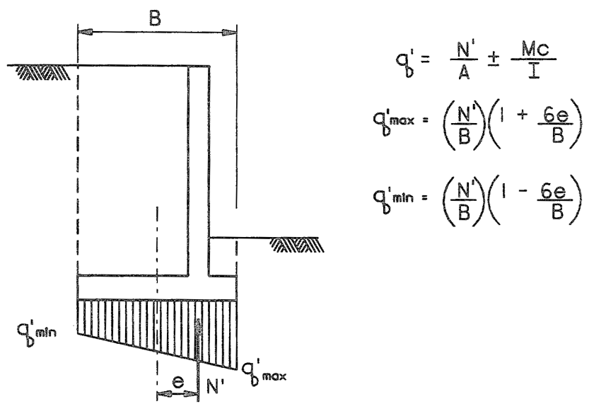
You may recall that, for a uniform pressure distribution, the load is in the middle of the distribution. If a shallow foundation is loaded concentrically, the load is through the centroid, and this is the case. That is designated by the centreline. If the load is concentric, the eccentricity e = 0 and the two pressures q’min and q’max are both the same, as we see in the equations above, namely the load divided by the width of the foundation.
If the load is eccentric, e is nonzero. As e increases, q’max increases and q’min decreases. When we reach the point where e = B/6, q’min = 0. Beyond that point we get liftoff from one end of the foundation, which is generally not an acceptable result, especially since foundations cannot transmit tension between the soil and the foundation. As long as -B/6 < e < B/6, both q’min and q’max are positive and at least this criterion is met. This region is referred to as the “middle third” and is crucual to the success of shallow foundations.
Eccentricity in loads is not strictly the result of off-centroid loads. It can also be due to a moment on the foundation, in which case e = M/N’ (without any other factors to make the load eccentric.)
If we look at the diagram above, there’s a similarity between that and the “ramped” loads we see bearing on retaining walls, the result of increasing vertical pressure (and by extension horizontal pressure) on the wall with increasing depth. Traditionally in retaining walls we divide such a ramped load up into a “rectangular” portion (constant) and a “triangular” portion (zero at one end, nonzero at the other.) But in reality we can develop a simple expression that is valid for linearly varying loads with non-negative pressures.
Consider the foundation above. It can be shown that the resultant force on the foundation due to the resisting pressure of the soil is given by the equation
(1)
or, more simply the average of the end pressures times the length of the foundation/wall section/beam. It can be shown that, if we define
(2)
Then the distance from the end with to the location of the resultant is
(3)
For the case of the triangle load () and for the uniform load () , as we know. If we subtract the two we get the maximum eccentricity , which we know defines the middle third.
So to not leave out the retaining wall and beam people, let’s consider the following example of sheet pile design using Pile Buck’s SPW911 software.
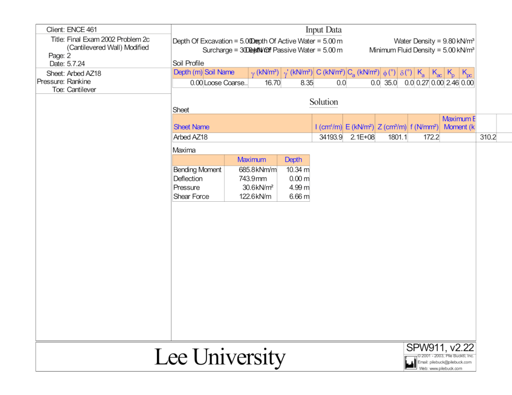
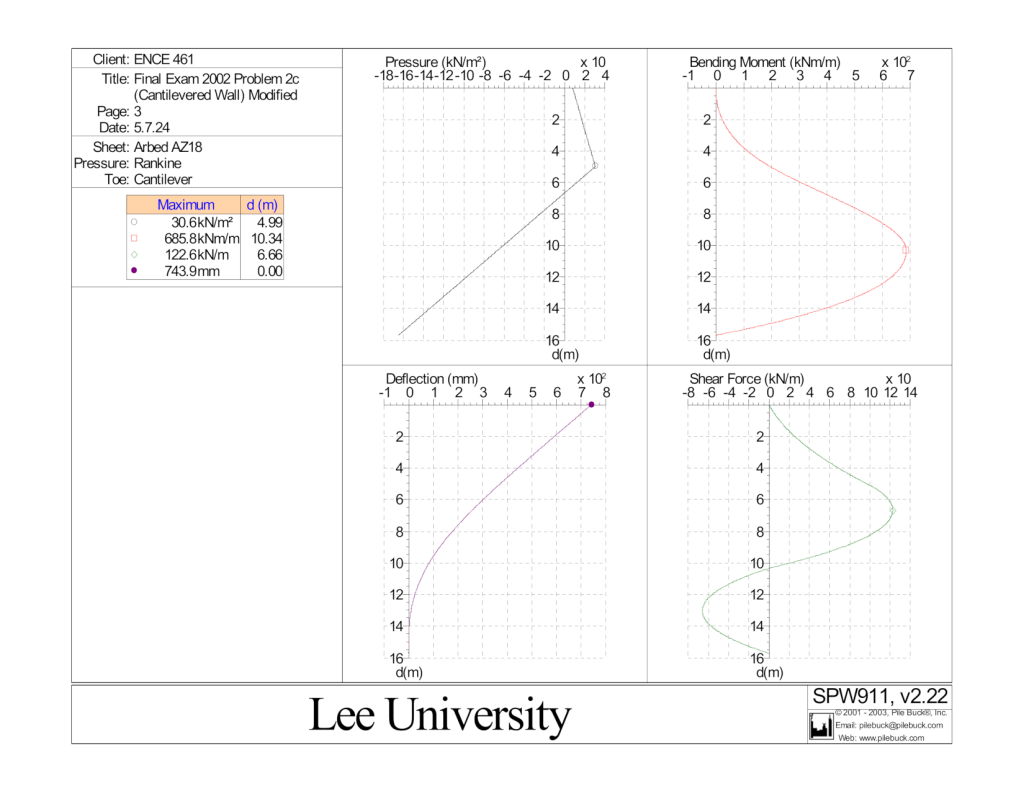
We’ll concentrate on the part which is above the dredge line, a length of 5 m. In this region there is only active pressure on the soil side of the wall; because of the 30 kPa surcharge at the surface, the load has a trapezoidal shape. Without going into the geotechnics of retaining walls (which you can review in the post Foundation Design and Analysis: Retaining Walls, Concrete Gravity Retaining Walls) the lateral pressure at the top of the wall is 8.2 kPa (from the table) and at the dredge line 30.6 kPa (from the main graphic, the maximum pressure.) We can thus say the following:
From Equation (2), adjusting the notation for retaining walls, .
From Equation (3), again adjusting the notation, from the top of the wall (smaller pressure,) or 2.02 m from the dredge line.
By Equation (1), the magnitude of the resultant (that’s metre of horizontal wall.) A free-body diagram of the upper 5 m of the wall tells us that, since we’ve replaced a distributed load with a resultant, the shear at the dredge line should be the same. Looking at the table, at 4.97 m from the top, the shear , which is very close.
Same free-body diagram shows us that the moment in the sheeting at the dredge line should be the resultant force times the distance from the resultant to the dredge line. Thus the moment . This too compares favourably with the moment at 4.97 m from the top, which is
It’s possible to do everything with resultants instead of distributed load integration, but for situations like this it’s easier to do the integration. With numerical methods such as SPW 911 uses, the wall is divided up into finite differences and each difference can be considered a beam, the results summed up and the pressures reduced to resultants. Resultants are very useful for determining boundary conditions like the shear and moment at supports. As noted in this post, if resultants are always used in place of distributed loads, the shears and moments will be conservative, unacceptably so in some cases.
Most all loads in geotechnical engineering are distributed loads, because they are the results of earth pressures, either horizontal (lateral) or vertical. Although most of these are either constant or ramped linear, the math with these gets complicated fast. In the past this was a major problem for geotechnical engineers armed with slide rules. The resultant is one way of simplifying the computations, and at the same time it offers better understanding of how earth pressures either load a structure or support it.
Let’s start with a definition: for most geotechnical problems, a resultant is a point load which is used to represent a distributed load. In general statics, the definition is broader, but this is what we’re going to discuss here. To accomplish this such a resultant must meet two criteria:
It must have the same total load as the distributed load.
It most pass through the centroid of the distributed load.
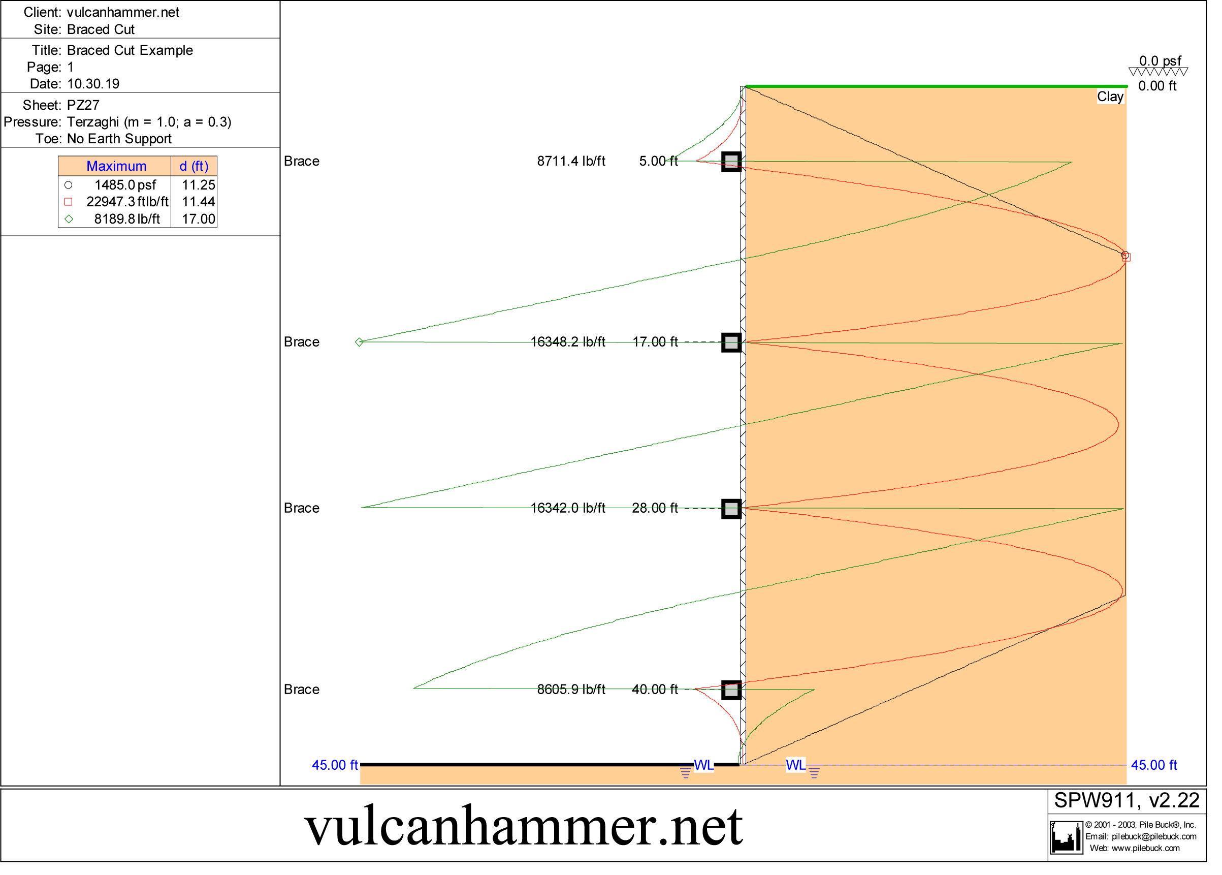
The example we’ll use here is from a previous post on braced cut analysis, a subject that has buffaloed many of my students over the years. The software layout of the wall, earth pressure loads, shears and moments is shown below.
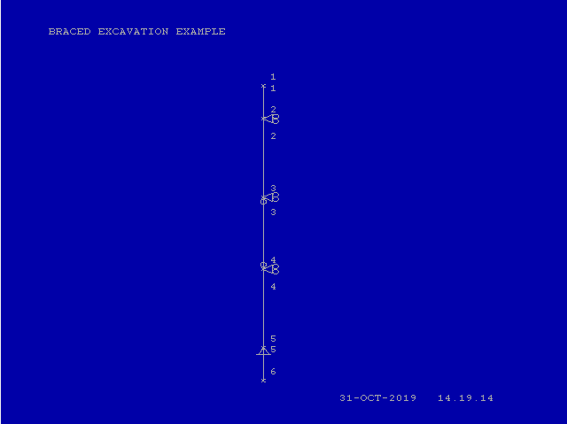
Using CFRAME to focus on the beam mechanics of the problem, first we will look at the model itself.
The basic layout of the model. The model is simply supported at all braces. Additionally–and this is one reason we wanted to use CFRAME–the central element 3 was additionally pinned at the ends to simulate Terzaghi and Peck’s original intent for the method.
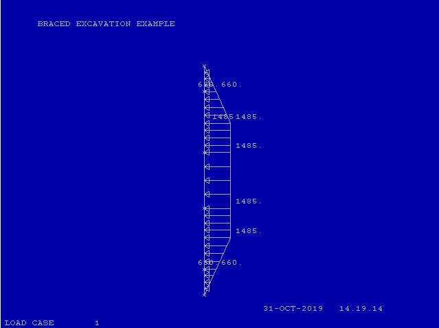
The distributed loading is then shown below.
The pressure distribution on the model, replicating that Terzaghi and Peck distribution for stiff clays.
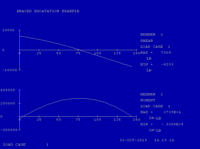
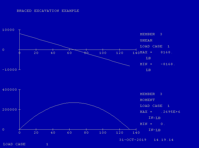
Let’s start with the easy section: the portion of the wall between 17′ and 28′ below the top of the wall (Element 3, between Nodes 3 and 4, shown in the basic layout.) As noted above, the beam has a distributed uniform of 1485 psf, or for our purposes 1485 lb/ft/ft of wall (vertical) and is simply supported on both ends. With this load the shear and moment looks like this, taken from the CFRAME program:
The way Terzaghi and Peck set this method forth, the beams at the top and bottom of the wall would be considered to be cantilever beams and the rest simply supported beams. This turns the whole problem into a statically determinate one, necessary to simplify the calculations. The diagram above shows a reaction of 8168 lbs. at each end, a maximum moment of 269,500 in-lb at the centre, and zero moment at the supports (due to the simply supported assumption.)
We could obtain this result by hand calculations. First, the reactions at the supports are given by the formula
(1)
which is the same as above. The maximum moment is given by the equation
(2)
which is also the same as above.
Note: one of my students got very put out with me because I had the bad taste to say that these formulas were in the "steel book," the AISC Steel Construction Manual. While I realise that it's hard to find anything in the steel book, they are there, and have been since the days I first used it at the Special Products Division.
Now let’s replace the distributed load by a resultant point load. Since the load is uniformly distributed, the centroid is at the centre of the beam. The resultant is
(3)
The reactions are computed by symmetry as follows:
(4)
and the maximum moment (at the centre of the beam) is
(5)
The reactions at the braces are the same. Thus, for the design of the braces, the methods give the same result. The maximum moment from the resultant, however, is twice the moment from a point load resultant. In practice one could deal with this problem by a) assuming the uncertainty in the earth loads justifies the conservatism of the resultant, b) scaling down the anticipated moment by noting the differences between the two (which are in turn the result of the statics of simply supported beams) or c) a combination of the two. In any case the need to use a resultant here isn’t great because of the uniform load.
Things get more complicated when we consider the second segment from the top, from 5′ to 17′. This 12′ long segment has the following pressure distribution:
At the top end of the beam, the pressure is 660 psf.
The pressure ramps up linearly to the maximum pressure of 1485 psf at a point 6.25′ from the end of the beam.
From this point until the bottom end of the beam 12′ from the top the pressure is uniform at 1485 psf.
Although it’s possible to get resultants from ramped load, it’s easier to divide a ramped load into a constant portion (minimum pressure) and a triangle load from zero to the difference between the minimum and maximum pressures. That being the case, the three regions are as follows, with their resultants:
The upper uniform region has a pressure of 660 psf and a length of 6.25′, thus its resultant is (660)(6.25) = 4125 lb/ft
The triangular region has a maximum pressure of 1485-660=825 psf, thus its resultant is (825)(6.25)/2 = 2578 lb/ft. The division by 2 is because it’s a triangle load.
The lower uniform region has a pressure of 1485 psf and a length of 12-6.25 = 5.75′, thus its resultant is (1485)(5.75) = 8539 lb/ft.
The location of these resultants is as follows:
The upper uniform region is half the length of the region, thus it is 6.25/2 = 3.125′ from the top end.
The upper triangular region is two-thirds the length of the region, thus it is 2*6.25/3 = 4.17′ from the top end
The lower uniform is the length of the upper region plus half the length of the lower region, thus it is 6.25 + 5.75/2 = 9.125′.
The reactions for a point load at any point in the beam are given by the equation
(6)
(7)
The variable k is the ratio of the distance from the top end of the resultant to the total beam length. We can add the contribution from each resultant to obtain total reactions.
Resultant
Fres, lb/ft
Location from top, ft
k
R1
R2
1
4125
3.125
0.26
3053
1073
2
2578
4.17
0.35
1676
902
3
8539
9.125
0.76
2046
6493
Total
15,242
6775
8468
It can be shown that the sum of the reactions is the same as the sum of the resultants within rounding error, as should be the case.
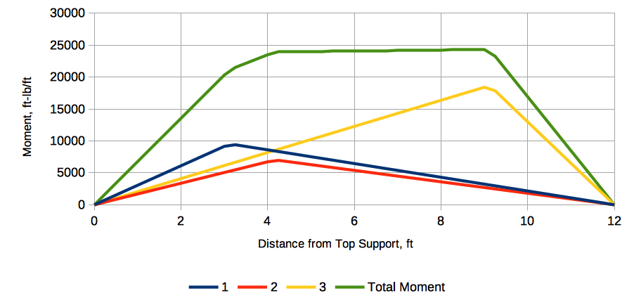
The maximum moment is a little more complicated. For any point load on a simply supported beam, the moment begins at zero at the support, linearly rises to a maximum of , and then linearly declines to zero at the opposite support. This means that each moment distribution needs to be determined at many points and then the result summed at each point to insure that the maximum moment is identified. The spreadsheet implementation of this is here and you can see the moment distribution for each resultant and their sums below. The maximum moment is 24,322 ft-lbs/ft = 291,869 in-lbs/ft.
Now let’s compare this with the CFRAME results, which took into consideration distributed loads. Hand calculations for distributed loads are fairly involved.
We’ll start with the moment. The maximum moment from CFRAME (273,900 in-lb/ft) is a little smaller that that which is predicted by the resultants. This is expected; the more resultants the load is divided into, the closer to the distributed load result the moment will become.
With the reactions, the sum of the reactions shown in CFRAME is identical to those from the resultant method; however, the reactions themselves are different. That’s because it is not possible to accurately reproduce a simply supported beam for Segment 2 and have a cantilever beam for Segment 1. In CFRAME we are forced to use a continuous beam from the top to the second brace (17′) and simply support them at both points. Note carefully that the moment at the left (top) end of the beam is nonzero, which is not the case with a simply supported beam. This illustrates that, from a structural standpoint, the method of Terzaghi and Peck for braced cuts is artificial, although it is possible to combine Segments 1 and 2 and do hand calculations for these with resultants.
It’s worth noting that the brace loads using SPW911 at 17′ and 28′ are 16,340 lb/ft of wall. If we use the resultant method, the brace loads (the structure is symmetric) should be 8468 + 8168 = 16,636 lb/ft and using CFRAME 8233 + 8168 = 16,401, neither of which are identical to SPW 911. This is a good illustration of the care you need to take when evaluating computer generated results.
Nevertheless, I think the use of resultants is adequately illustrated by this example. Perhaps in the future more examples of resultants can be given.
Last Thursday evening the College of Engineering of the University of Tennessee at Chattanooga presented me with a couple of awards. Outstanding Lecturer/Adjunct Teaching Award, Department of Mechanical Engineering, College of Engineering and Computer Science, University of Tennessee at Chattanooga I find myself disparaging some of my activities as “award-losing,” and they certainly are, but […]


 (1)
(1) of the foundation/wall section/beam. It can be shown that, if we define
 (2)
(2) to the location of the resultant is
 (3)
(3) )
)  and for the uniform load (
 )
)  , as we know. If we subtract the two we get the maximum eccentricity
  , which we know defines the middle third.

 .
. from the top of the wall (smaller pressure,) or 2.02 m from the dredge line.
  (that’s metre of horizontal wall.) A free-body diagram of the upper 5 m of the wall tells us that, since we’ve replaced a distributed load with a resultant, the shear at the dredge line should be the same. Looking at the table, at 4.97 m from the top, the shear
  , which is very close.
 . This too compares favourably with the moment at 4.97 m from the top, which is
 (1)
(1) (2)
(2) (3)
(3) (4)
(4) (5)
(5) (6)
(6) (7)
(7) , and then linearly declines to zero at the opposite support. This means that each moment distribution needs to be determined at many points and then the result summed at each point to insure that the maximum moment is identified.