vulcanhammer.net

How Those “Award-Winning” Lab Videos Came into Being — Chet Aero Marine

Posted on 24 October 2021 by Don Warrington

Last Thursday evening the College of Engineering of the University of Tennessee at Chattanooga presented me with a couple of awards. Outstanding Lecturer/Adjunct Teaching Award, Department of Mechanical Engineering, College of Engineering and Computer Science, University of Tennessee at Chattanooga I find myself disparaging some of my activities as “award-losing,” and they certainly are, but […]
How Those “Award-Winning” Lab Videos Came into Being — Chet Aero Marine

Geotechnical Engineering

Rankine and Coulomb Earth Pressure Coefficients

Posted on 28 September 202112 April 2025 by Don Warrington

For retaining walls, computing these is important; but the textbooks and reference books are frequently confusing and sometimes wrong. These formulae, derived using Maple, should clear up a few things, although they’re a) not always in the format you’re used to and b) subject to the Terms and Conditions of this site.

Let’s start with a diagram and the basic Coulomb formulae, from NAVFAC DM 7.02, shown above. It’s important for to have a nomenclature chart for any lateral earth pressure coefficient formulae.

Coulomb Active Coefficients

All angles nonzero:

$K_{{a}}=\left (\cos(-\phi+\theta)\right )^{2}\left (\cos(\theta)\right )^{-2}\left (\cos(\theta+\delta)\right )^{-1}\left (1+\sqrt {-{\frac {\sin(\phi+\delta)\sin(-\phi+\beta)}{\cos(\theta+\delta)\cos(\theta-\beta)}}}\right )^{-2}$ (1a)

Vertical Wall:

$K_{{a}}=\left (\cos(\phi)\right )^{2}\left (\cos(\delta)\right )^{-1}\left (1+\sqrt {{\frac {\sin(\phi+\delta)\sin(\phi-\beta)}{\cos(\delta)\cos(\beta)}}}\right )^{-2}$ (1b)

Level Backfill:

$K_{{a}}=\left (\cos(-\phi+\theta)\right )^{2}\left (\cos(\theta)\right )^{-2}\left (\cos(\theta+\delta)\right )^{-1}\left (1+\sqrt {{\frac {\sin(\phi+\delta)\sin(\phi)}{\cos(\theta+\delta)\cos(\theta)}}}\right )^{-2}$ (1c)

Vertical Wall and Level Backfill:

$K_{{a}}={\frac {\left (\cos(\phi)\right )^{2}}{\left (\sqrt {\cos(\delta)}+\sqrt {\sin(\phi+\delta)}\sqrt {\sin(\phi)}\right )^{2}}}$ (1d)

Coulomb Passive Coefficients

All angles nonzero:

$K_{{p}}=\left (\cos(\phi+\theta)\right )^{2}\left (\cos(\theta)\right)^{-2}\left (\cos(\theta-\delta)\right )^{-1}\left (1-\sqrt {{\frac {\sin(\phi+\delta)\sin(\phi+\beta)}{\cos(\theta-\delta)\cos(\theta-\beta)}}}\right )^{-2}$ (1e)

Vertical Wall:

$K_{{p}}={\frac {\left (\cos(\phi)\right )^{2}\cos(\beta)}{\cos(\beta)\cos(\delta)-2\,\sqrt {\cos(\beta)}\sqrt {\cos(\delta)}\sqrt {\sin(\phi+\beta)}\sqrt {\sin(\phi+\delta)}+\sin(\phi+\beta)\sin(\phi+\delta)}}$ (1f)

Level Backfill:

$K_{{p}}={\frac {\left (\cos(\phi+\theta)\right )^{2}}{\cos(\theta)\left (\cos(\theta)\cos(\theta-\delta)-2\,\sqrt {\cos(\theta)}\sqrt {\cos(\theta-\delta)}\sqrt {\sin(\phi+\delta)}\sqrt {\sin(\phi)}+\sin(\phi+\delta)\sin(\phi)\right )}}$ (1g)

Vertical Wall and Level Backfill:

$K_{{p}}=-{\frac {\left (\cos(\phi)\right )^{2}}{-\cos(\delta)+2\,\sqrt {\cos(\delta)}\sqrt {\sin(\phi+\delta)}\sqrt {\sin(\phi)}-\sin(\phi+\delta)\sin(\phi)}}$ (1h)

Rankine Active Coefficients

These were derived assuming that Rankine coefficients are the same as their Coulomb counterparts except for $\delta = 0$ ). This is strictly speaking not the case and will be discussed in detail below.

Sloping Wall and Backfill:

$K_{{a}}=\left (\cos(\phi-\theta)\right )^{2}\left (\cos(\theta)\right)^{-3}\left (1+\sqrt {{\frac {\sin(\phi)\sin(\phi-\beta)}{\cos(\theta)\cos(\theta-\beta)}}}\right )^{-2}$ (2a)

Vertical Wall:

$K_{{a}}=\left (\cos(\phi)\right )^{2}\left (1+\sqrt {{\frac {\sin(\phi)\sin(\phi-\beta)}{\cos(\beta)}}}\right )^{-2}$ (2b)

Level Backfill:

$K_{{a}}=\left (\cos(\phi-\theta)\right )^{2}\left (\cos(\theta)\right)^{-3}\left (1+\sqrt {{\frac {\left (\sin(\phi)\right )^{2}}{\left (\cos(\theta)\right )^{2}}}}\right )^{-2}$ (2c)

Vertical Wall and Level Backfill:

$K_{{a}}={\frac {\left (\cos(\phi)\right )^{2}}{\left (1+\sin(\phi)\right )^{2}}}$ (2d)

Rankine Passive Coefficients

$K_{{p}}=\left (\cos(\phi+\theta)\right )^{2}\left (\cos(\theta)\right)^{-3}\left (1-\sqrt {{\frac {\sin(\phi)\sin(\phi+\beta)}{\cos(\theta)\cos(\theta-\beta)}}}\right )^{-2}$ (2e)

Vertical Wall:

$K_{{p}}=-{\frac {\left (\cos(\phi)\right )^{2}\cos(\beta)}{-\cos(\beta)+2\,\sqrt {\cos(\beta)}\sqrt {\sin(\phi+\beta)}\sqrt {\sin(\phi)}-\sin(\phi+\beta)\sin(\phi)}}$ (2f)

Level Backfill:

$K_{{p}}=-{\frac {\left (\cos(\phi+\theta)\right )^{2}}{\cos(\theta)\left (-\left (\cos(\theta)\right )^{2}+2\,\cos(\theta)\sin(\phi)-1+\left (\cos(\phi)\right )^{2}\right )}}$ (2g)

Vertical Wall and Level Backfill:

$K_{{p}}={\frac {\left (\cos(\phi)\right )^{2}}{\left (-1+\sin(\phi)\right )^{2}}}$ (2h)

The Origin of Rankine Earth Pressure Coefficients

It is a matter of record that Rankine earth pressure coefficients were derived from a combination of Mohr-Coulomb failure theory and the effect of wall movement on the horizontal earth pressure. The physical manifestation of the theory is illustrated at the right, based on tests which have been run over the years.

OTOH, Coulomb earth pressures were derived from the static equilibrium of a soil wedge (with a failure surface, see diagram at left.)

The thing that has confused the issue is that, for the case of level backfill, vertical wall and no wall friction, the results of Equations (2d) and (2h) are identical with the Rankine theory results as originally derived. This equivalence is doubtless more than fortuitous but it does not necessarily extend upwards to the other cases.

This has been recognised for a long time. For the case of the vertical wall and sloping backfill, the application of “conjugate stresses” (Hough, 1970) as opposed to principal stresses results in the following “Rankine” earth pressure coefficient:

$K_{{a}}={\frac {\cos(\beta)\left (\cos(\beta)-\sqrt {\left (\cos(\beta)\right )^{2}-\left (\cos(\phi)\right )^{2}}\right )}{\cos(\beta)+\sqrt {\left (\cos(\beta)\right )^{2}-\left (\cos(\phi)\right )^{2}}}}$ (3)

and its passive counterpart

$K_{{a}}={\frac {\cos(\beta)\left (\cos(\beta)+\sqrt {\left (\cos(\beta)\right )^{2}-\left (\cos(\phi)\right )^{2}}\right )}{\cos(\beta)-\sqrt {\left (\cos(\beta)\right )^{2}-\left (\cos(\phi)\right )^{2}}}}$ (4)

Ebeling and Morrison (1992) note the following about Equation (3):

The Rankine active earth pressure coefficient for a dry frictional backfill inclined at an angle $\beta$ from horizontal is determined by computing the resultant forces acting on vertical planes within an infinite slope verging on instability, as described by Terzaghi (1943) and Taylor (1948).

Equations (2b) and (3) reduce to Equation (2d) and Equations (2f) and (4) reduce to Equation (2h) when $\beta = 0$ .

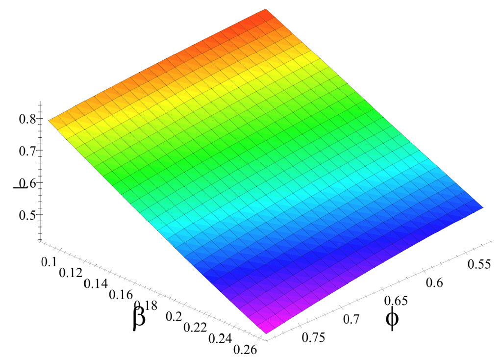
A quick comparison was made by dividing the right hand side of Equation (3, numerator) by the right hand side of Equation (2b, denominator.) A survey of the results are shown below. The angles are shown on the x- and y-axes in radians; the friction angle $\phi$ varies from 30 to 45 degrees and the backfill angle $\beta$ varies from 5 to 15 degrees. The result shows that the Terzaghi and Taylor (an interesting combination to say the least) coefficients are slightly lower than the Coulomb derived coefficients.

It’s a completely different story with the passive coefficients; dividing the right hand side of Equation (4) by the right hand side of Equation (2f) with the same angle ranges as above gives us the following result:

As an interesting side note, if we take a test case of φ = 30 deg. and β = 10 deg., the passive coefficient using Equation (4) is actually less than the one for level backfill!

This is a topic that deserves further investigation; however, extending Rankine theory using Coulomb wedge theory without wall friction has merit for those applications (such as vinyl or fibreglass sheet piling) where inclusion of wall friction is inappropriate to the application.

References

Ebeling, R.M., and Morrison, E.E. Jr. (1992) The Seismic Design of Waterfront Retaining Structures. Technical Report ITL-92-11. Vicksburg, MS: U.S. Army Waterways Experiment Station.

Hough, B.K. (1970) Basic Soils Engineering. Second Edition. New York: The Ronald Press Company.

Vulcan and Sheet Piling — vulcanhammer.info

Posted on 21 September 2021 by Don Warrington

The development of sheet piling and the Warrington-Vulcan hammers was about the same time (along with concrete piles, other types of steel piles, and the Engineering News Formula.) The years leading up to World War I were ones of rapid development in the marine construction and deep foundation industries, and Vulcan was in the middle […]
Vulcan and Sheet Piling — vulcanhammer.info

Geotechnical Engineering

The Difference Between Flamant’s and Terzaghi’s Solution for Line Loads Behind Retaining Walls

Posted on 9 September 2021 by Don Warrington

Generally speaking, in Soil Mechanics courses elastic solutions on semi-infinite half spaces are presented to allow the geotechincal engineer to estimate the stresses induced in a soil by a load at the surface. Also presented in Soil Mechanics courses are charts and equations to estimate the lateral pressures on retaining walls induced by vertical loads on the surface behind the retaining walls. How either of these came into being is generally not explained; additionally, the fact that they are related is not explained either. The purpose of this article is to explain that relationship and, in the case of the retaining walls, how the original equations have been modified to suit experimental data. For simplicity’s sake, the discussed will be restricted to line loads.

The Original Equations: Flamant

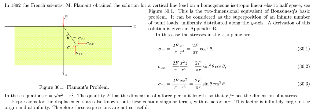
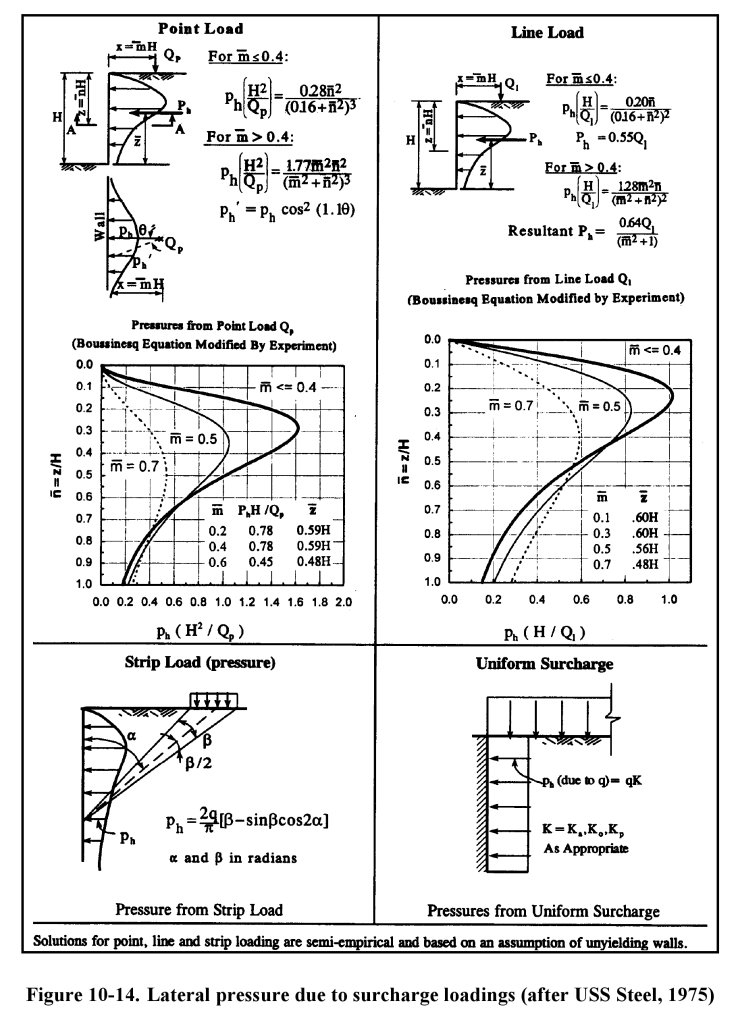
As pointed out by Verruijt, the original equation for the stresses (vertical, horizontal and shear) were first set forth by Flamant in 1892. The equations are shown below.

Flamant Solution for a Line Load on a Semi-Infinite Elastic Medium, from Verruijt

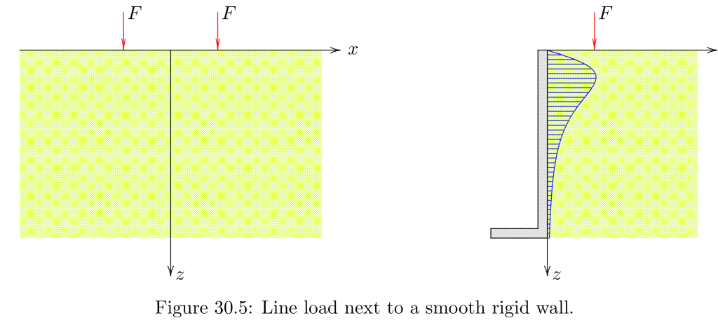
The derivation of this equation can be found here or in Verruijt. Note carefully that the vertical load induces stresses in the horizontal direction (and in shear) as well as the vertical direction.

Verruijt then shows the following:

Mirror Flamant Loads on either side of an arbitrary dividing line and the computation of stress against a rigid wall.

Basically, by static equilibrium, if you replace the left half of the two mirrored loads (on the left) with a rigid wall, the horizontal stresses would be the same on the centre axis/wall as induced by two line loads. The resulting stresses and the resultant for the stress distribution are given below.

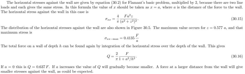
Flamant’s Equation for Horizontal Stresses Against a Rigid Wall, Including the resultants

The Modified Equations: Terzaghi

Generally, however, these equations are not presented in books such as DM 7, Sheet Pile Design by Pile Buck or others in this exact form. The following chart (frequently copied) comes from the Soils and Foundations Manual:

The line load is in the upper right hand corner. For values of m (the ratio of the distance from the line load to the wall over the height of the wall) greater than or equal to 0.4, the two results are the same. For those less than that, they are different. (In Verruijt’s notation, m = a/z.) The difference is because most books use the formulation of Terzaghi (1954). He explains the difference as follows:

However, the application of the line load tends to produce a lateral deflection of the vertical section, and the flexural rigidity of the bulkhead interferes with that deflection…However, for values smaller than (m=)0.4, the discrepancy between observed and computed values increases with decreasing values values of m…
From Terzaghi, K. (1954) “Anchored Bulkheads.” Transactions of the American Society of Civil Engineers, Vol. 119, Issue 1.

The whole issue of the flexibility of the retaining wall has been the chief complicating factor in this discussion, going back to Spangler’s tests in the 1930’s.

Comparing the Two Solutions

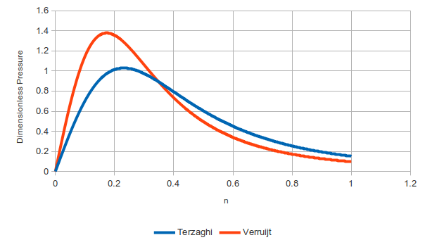
As an illustration, consider the pressure distribution situation when m=0.3:

Comparison of Flamant/Verruijt and Terzaghi Solutions for Line Load Pressures, m = 0.3

The pressures have been made dimensionless for generalisation. The Flamant solution comes to a higher peak nearer to the surface but falls off more rapidly down the wall. Terzaghi’s solution is more evenly distributed.

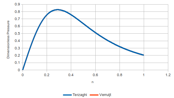
Now consider the situation at m=0.5:

Comparison of Flamant/Verruijt and Terzaghi Solutions for Line Load Pressures, m = 0.5

The two are identical in this range.

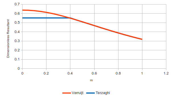
We can also consider the resultants as well:

Comparison of Flamant/Verruijt and Terzaghi Solutions for Line Load Resultants

The y-axis is made dimensionless by dividing the resultant by the vertical line load. For values of m less than or equal to 0.4, the results are different; for greater, they are the same.

In general, we can say that Flamant’s original formulation is more conservative. In the event that a deeper understanding of the interaction of surface loads with a retaining wall is desired, a finite element analysis needs to be done.

Soil Mechanics

Fatal Landslide Triggered by Hurricane Ida

Posted on 3 September 2021 by Don Warrington

A portion of the embankment on MS26 in George County Mississippi failed after heavy rains and flooding caused by Hurricane Ida. It created a hole about 20 feet deep and 50 feet across late on Monday night, and I can imagine it was difficult for motorists to see until it was too late. There were […]
Fatal Landslide Triggered by Hurricane Ida