vulcanhammer.net

Going Around in Circles for Rigid and Flexible Foundations

Posted on 30 May 20224 April 2023 by Don Warrington

In an earlier post Analytical Boussinesq Solutions for Strip, Square and Rectangular Loads, we discussed elastic solutions for these types of foundations. Most of the results shown were for perfectly elastic foundations. In this post we will concentrate on a) circular foundations and b) the difference between rigid and elastic foundations, and those which find themselves in between.

Circular Foundations

Engineers have been familiar with charts such as this, from NAVFAC DM 7.01:

The influence coefficients (see diagram above) for the vertical, horizontal and shear stresses respectively directly under the centre of the load (x = 0) are not difficult to compute, being

$I_z = 1 - \frac{z^3}{(z^2+r^2)^\frac{3}{2}}$
$I_r = (1+\nu)\frac{z}{\sqrt{z^2+b^2}} - \frac{1}{2}(1 - \frac{z^3}{(z^2+r^2)^\frac{3}{2}})$
$I_{zr} = 0$

For just about everywhere else (except for the edge) closed form solutions are hard to come by. Why is this? Because, for most every other point, the solution for the influence coefficients involves the use of elliptical integrals. An illustration of the values of these is shown below.

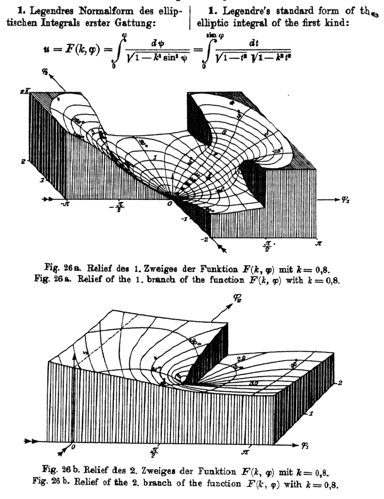
Examples of elliptical integrals (from Jahnke and Emde (1945))

Although mathematical packages such as Maple and Matlab are certainly capable of evaluating these, they are still not the common companions of engineers. Fortunately most of the questions about the stresses under circular foundations centre (sorry!) around the point under x = 0, so the above formulae are useful.

Foundations Rigid and Flexible

Up to this point, we’ve considered for the most part the response of the soil–both stress and deflection–to a purely flexible foundation. For these foundations at the soil-foundation interface the pressure exerted on the foundation and the pressure the foundation exerts on the soil is the same. If there is any rigidity in the foundation–and virtually any foundation has some–then both deflections and stresses in the foundation are redistributed.

It’s probably useful to note that, for deflections in general, the formula we use is

$s = \frac{\omega p b (1-\nu^2)}{E}$

where

$s =$ settlement of the foundation at the point of interest
$\omega = I =$ influence factor
$p =$ uniform pressure on the foundation
$b = B =$ smaller dimension of rectangle or dimension of square side
$\nu =$ Poisson’s Ratio of the soil
$E =$ Modulus of elasticity of the soil

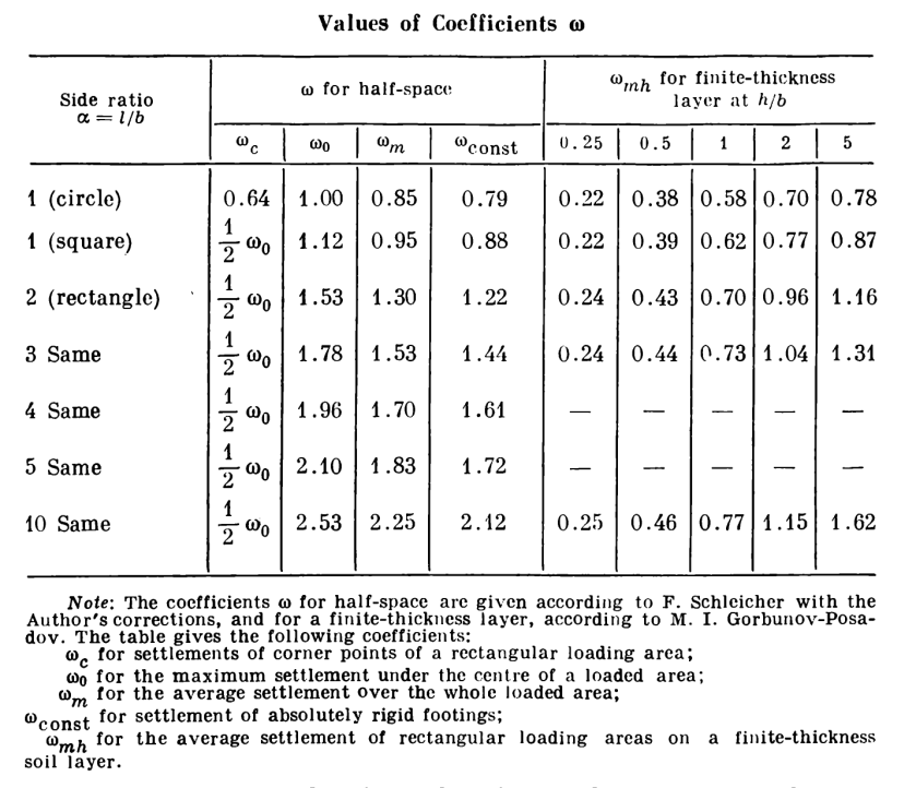
The values for $\omega$ are given below.

Values for the influence coefficients omega (from Tsytovich (1976))

Turning to the flexible circular foundation, the value for $\omega$ for all of the radii can be computed using the formula (Timoshenko and Goodier (1951)):

$\omega=\frac{2}{\pi}\,\int_{0}^{1/2\,\pi}\!\sqrt{1-{\frac{{x}^{2}\left(\sin(\psi)\right)^{2}}{{r}^{2}}}}{d\psi}$

This still has a complete elliptical integral of the second kind, but it more manageable. It can be solved by applying the trapezoidal rule and using small integration increments over the interval. Values for $\omega$ for ratios of various values of x (see diagram above) to the actual radius of the circle are shown below.

Although many elastic calculations assume the flexible foundation, as noted earlier in reality foundations have rigidity. For a perfectly rigid foundation, the deflection of the entire foundation under a concentric load is uniform. The effect of this on the stresses can be seen below.

Diagrams of contact pressures a) under an absolutely rigid foundation, b) under foundations of various flexibilities. (From Tsytovich (1976))

For the foundation in (a), if it is a circular foundation, the vertical stresses at the base can be computed by the formula

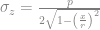
$\sigma_{z}=\frac{p}{2\sqrt{1-\left(\frac{x}{r}\right)^{2}}}$

At the corners of the foundation, the stresses are theoretically infinite. This means that the lower bound solution for such a foundation is zero stress. In reality it is reasonable to assume that a) no foundation is perfectly rigid and b) the soil will proceed into plastic deformation, which will redistribute the stresses.

It is interesting to note that, for the strip loads we discussed previously, the distribution for a rigid strip is similar to the circle, thus

$\sigma_{z}=\frac{2p}{\pi \sqrt{1-\left(\frac{2y}{b}\right)^{2}}}$

where the notation is as it was in that discussion.

The figure (b) above shows different vertical stress distributions for different flexibility ratios, given by the variable $\Gamma$ . This can be approximated by the formula (Tsytovich (1976))

$\Gamma \cong 10\frac{E_s l^3}{E_f h_1^3}$

where

$E_s =$ modulus of elasticity of the soil
$l =$ half-width of the foundation, shown above
$E_f =$ modulus of elasticity of the foundation
$h_1 =$ height of the foundation

To get a better approximation would require plate theory, where the mathematics are very involved; an example of this, using a pile toe where the circle is loaded around the edge, can be found here.

The rigidity of the foundation also influences the distribution of stresses under the foundation, as shown below.

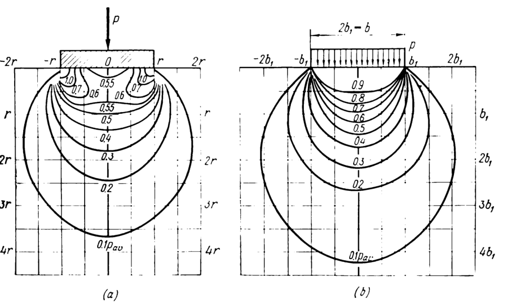
Isobars in Soil under Foundations a)absolutely rigid foundation, b)flexible foundation (from Tsytovich (1976))

There’s certainly life beyond elastic theory. In reality the type of soil affects the distribution of contact pressure on the foundation, even with a uniformly loaded foundation, as shown below.

Contact pressure under a)rigid footings and b)elastic foundation on an elastic half-space (from NAVFAC DM 7.01 (1986))

The clay distribution most resembles that of an elastic response of a soil with a rigid footing, as discussed earlier. The purely flexible foundation will have the same uniform reaction as the load, as noted earlier.

Other Sources

Foster, C.R. and Ahlvin, P.G. (1954) “Stresses and Deflections Induced by Uniform Circular Load.” Highway Research Board Proceedings, Highway Research Board, Washington, DC.
Jahnke, E. and Emde, F. (1945) Tables of Functions with Formulae and Curves. New York: Dover Publishers.
Timoshenko, S., and Goodier, J.N. (1951) Theory of Elasticity. New York: McGraww-Hill Book Company, Inc.

Lower and Upper Bound Solutions for Bearing Capacity

Posted on 6 May 202215 October 2022 by Don Warrington

Although today we have finite element methods which can combine elastic and plastic components of soil response to loading, the use of lower and upper bound plasticity is important in enhancing our understanding of plasticity in soils and many of the methods we use in geotechnical design. This is an overview of both lower and upper bound solutions to the classic bearing capacity problem. Much of this presentation is drawn from Tsytovich (1976) but the equations have been re-derived and checked.

Definitions (from Verruijt)

Lower bound theorem.The true failure load is larger than the load corresponding to an equilibrium system.

Upper bound theorem.The true failure load is smaller than the load corresponding to a mechanism, if that load is determined using the virtual work principle.

For our purposes, since we’re assuming an elastic/perfectly plastic type of soil model, the lower bound solution is where the stress at some point reaches the elastic limit, while the upper bound solution has the stress fully plastic to the boundaries of the system, at which point the capacity of the system to resist further stress has been exhausted (reached its upper limit.)

Assumptions

Foundation is very rigid relative to the soil (for upper bound) and flexible relative to soil (lower bound.) With the latter, a rigid foundation produces infinite stresses at the edges, which means the lower bound solution is zero pressure in that case.
No sliding occurs between foundation and soil (rough foundation)
Applied load is compressive and applied vertically to the centroid of the foundation (upper bound) or uniformly (lower bound)
No applied moments present
Foundation is a strip footing (infinite length)
Soil beneath foundation is homogeneous semi-infinite mass. For the derivations here, we additionally assume that the properties of the soil above the base of the foundation are the same as those below it
Mohr-Coulomb model for soil
General shear failure mode is the governing mode
No soil consolidation occurs
Soil above bottom of foundation has no shear strength; is only a surcharge load against the overturning load
The effective stress of the soil weight acts in a hydrostatic fashion, i.e., the horizontal stresses are the same as the vertical ones.

These are fairly standard assumptions for basic bearing capacity theory; the “additions” from these are workarounds that have been developed. That includes the analysis of finite foundations (squares, rectangles, circles, etc.)

Theory of Elasticity of Infinite Strip Footings

Let us begin by considering the system below of a strip footing with a uniform load. The variables are defined in the figure.

Figure 1 Elastic Model of Stresses of Strip Loads (adapted from Tsytovich (1976))

It can be shown that the stresses at a point of interest can be defined as follows:

$\sigma_{{z}}={\frac {p\left (\alpha+\sin(\alpha)\cos(2\,\beta)\right )}{\pi }}$ (1)
$\sigma_{{y}}={\frac {p\left (\alpha-\sin(\alpha)\cos(2\,\beta)\right )}{\pi }}$ (2)
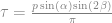
$\tau={\frac {p\sin(\alpha)\sin(2\,\beta)}{\pi }}$ (3)

It can also be shown that the principal axis of the stresses at the point are along a line in the middle of the angle $\alpha$ . This is the dashed line in the diagram above. Along this line the angle $\beta = 0$ (and thus $\frac{\alpha}{2}=-\beta'$ ) and the principal stresses due to the load become

$\sigma_{{1}}={\frac {p\left (\alpha+\sin(\alpha)\right )}{\pi }}$ (4)
$\sigma_{{3}}=-{\frac {p\left (-\alpha+\sin(\alpha)\right )}{\pi }}$ (5)

Lower Bound Solution

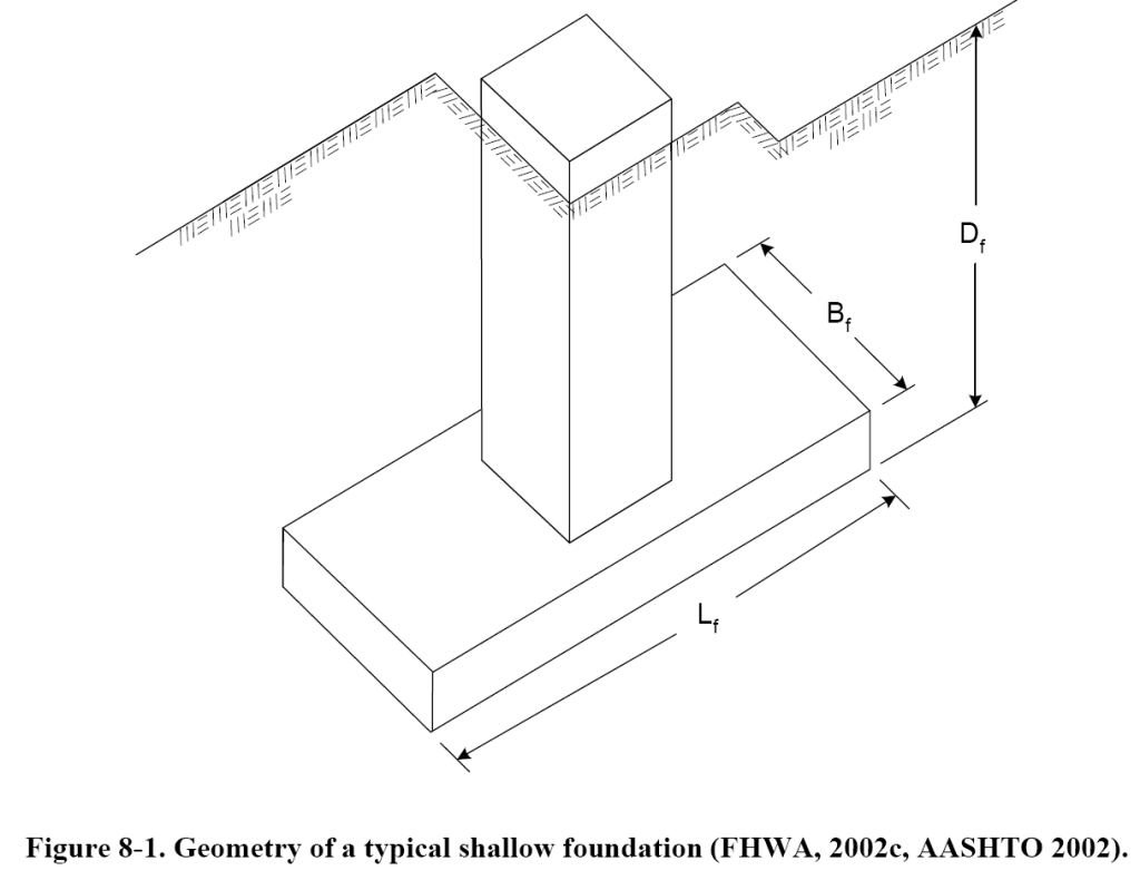
Shallow foundations are seldom built with the base of the foundation at the same elevation as the groundline. They are customarily built to a depth from the surface, as shown below.

Figure 2 Geometry and Nomenclature of a Typical Shallow Foundation (from Soils and Foundations Manual)

At this point, for analysis purposes, we transform the effect of the depth into an overburden stress, which is the product of the the unit weight of the soil $\gamma$ and the depth of the foundation base from the surface D (or h,) as shown below:

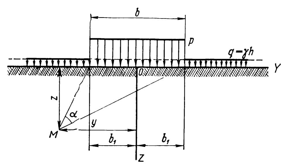
Figure 3 Strip Foundation with Surrounding Overburden (from Tsytovich (1976))

The effective stress at any point below the surface is given by the equation

$\sigma_{{0}}={\it \gamma}\,\left (h+z\right )$ (6)

At the point the hydrostatic stress assumption becomes important. The transformation from Equations (1-3) to (4-5) involved an axis rotation. Assuming the soil acts hydrostatically means that, no matter how we rotate the axis, the addition of the effective stress to the principal stress is independent of direction.

Doing just that yields the following:

$\sigma_{{1}}={\frac {\left (p-{\it \gamma}\,h\right )\left (\alpha+\sin(\alpha)\right )}{\pi }}+{\it \gamma}\,\left (h+z\right )$ (7)
$\sigma_{{3}}={\frac {\left (p-{\it \gamma}\,h\right )\left (\alpha-\sin(\alpha)\right )}{\pi }}+{\it \gamma}\,\left (h+z\right )$ (8)

At this point we state the failure function for Mohr-Coulomb theory:

$\sigma_{{1}}-\sigma_{{3}}-2\,c\cos(\phi)-\left (\sigma_{{1}}+\sigma_{{3}}\right )\sin(\phi)=0$ (9)

Substituting Equations (7) and (8) into Equation (9) yields

$-2\,{\frac {-p\sin(\alpha)+{\it \gamma}\,h\sin(\alpha)+c\cos(\phi)\pi+\sin(\phi)p\alpha-\sin(\phi){\it \gamma}\,h\alpha+\sin(\phi){\it \gamma}\,\pi \,h+\sin(\phi){\it \gamma}\,\pi \,z}{\pi }}=0$ (10)

Solving for z, we have

$z={\frac {p\sin(\alpha)}{\sin(\phi){\it \gamma}\,\pi }}-{\frac {h\sin(\alpha)}{\sin(\phi)\pi }}-{\frac {c\cos(\phi)}{\sin(\phi){\it \gamma}}}-{\frac {p\alpha}{{\it \gamma}\,\pi }}+{\frac {h\alpha}{\pi }}-h$ (11)

At this point we want to find the maximum value of z at which point plasticity first sets in. We do this by taking the derivative of z relative to $\alpha$ and setting it to zero, or

${\frac {p\cos(\alpha)}{\sin(\phi){\it \gamma}\,\pi }}-{\frac {h\cos(\alpha)}{\sin(\phi)\pi }}-{\frac {p}{{\it \gamma}\,\pi }}+{\frac {h}{\pi }}=0$ (12)

It can be shown that this condition is fulfilled when $\alpha = \frac{\pi}{2}$ . Substituting that value back into Equation (11) gives us the value of z at which point plasticity is first induced, or

$z_{{\max}}={\frac {p\cos(\phi)}{\sin(\phi){\it \gamma}\,\pi }}-{\frac{h\cos(\phi)}{\sin(\phi)\pi }}-{\frac {c\cos(\phi)}{\sin(\phi){\it \gamma}}}-1/2\,{\frac {p}{{\it \gamma}}}+{\frac {p\phi}{{\it \gamma}\,\pi }}-1/2\,h-{\frac {h\phi}{\pi }}$ (13)

If we solve for the pressure $p$ , that pressure will be in reality the critical pressure at which plasticity is first induced. Solving for that pressure,

$p_{{{\it cr}}}={\frac {2\,z_{{\max}}\sin(\phi){\it \gamma}\,\pi +2\,h\cos(\phi){\it \gamma}+2\,c\cos(\phi)\pi +\sin(\phi){\it \gamma}\,\pi\,h+2\,h\phi\,\sin(\phi){\it \gamma}}{2\,\cos(\phi)-\sin(\phi)\pi +2\,\phi\,\sin(\phi)}}$ (14)

At this point we need to face reality and note that, if the point we’re looking for is the point at which plastic deformation begins, then it cannot be at any depth other than the base of the foundation, or $z_{max} = 0$ . Making that final substitution yields at last

$p_{{{\it cr}}}={\frac {2\,h\cos(\phi){\it \gamma}+2\,c\cos(\phi)\pi +\sin(\phi){\it \gamma}\,\pi \,h+2\,h\phi\,\sin(\phi){\it \gamma}}{2\,\cos(\phi)-\sin(\phi)\pi +2\,\phi\,\sin(\phi)}}$ (15)

Upper Bound

The upper bound solution is a well-worn path in geotechnical engineering and only the highlights will be shown here.

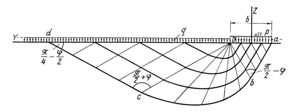
In 1920-1 Prandtl and Reissener solved the problem for a soil by neglecting its own weight, i.e., Equation (6) They determined that the failure pattern and surface can be represented by the following configuration.

Figure 3 Slip Lines and Failure Surface for Upper Bound Bearing Capacity Failure (from Tsytovich (1976))

They determined that the upper bound critical pressure was given by the equation

$p_{{{\it cr}}}={\frac {\left (q+c\cot(\phi)\right )\left (1+\sin(\phi)\right ){e^{\pi \,\tan(\phi)}}}{1-\sin(\phi)}}-c\cot(\phi)$ (16)

If we define

$N_{{q}}={\frac {\left (1+\sin(\phi)\right ){e^{\pi \,\tan(\phi)}}}{1-\sin(\phi)}}$ (17)

then

$p_{{{\it cr}}}=qN_{{q}}+c\cot(\phi)\left (N_{{q}}-1\right )$ (18)

If we further define

$N_{{c}}=\left (N_{{q}}-1\right )\cot(\phi)$ (19)

we have

$p_{{{\it cr}}}=qN_{{q}}+cN_{{c}}$ (20)

The only thing missing from this equation is the effect of the weight of the soil bearing on the failure surface at the bottom of the failure region shown in Figure 3, and thus the bearing capacity equation can be written thus:

$p_{{{\it cr}}}=qN_{{q}}+cN_{{c}}+1/2\,{\it \gamma}\,bN_{{{\it \gamma}}}$ (21)

where

$N_{{{\it \gamma}}}=2\,\left (N_{{q}}+1\right )\tan(\phi)$ (22)

This last bearing capacity factor has been the subject of variable solutions over the years; the one shown here is that of Vesić, which is enshrined in FHWA/AASHTO recommended practice. Verruijt discusses this issue in detail.

Worked Example

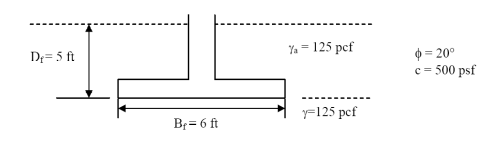
We can take an example from the Soils and Foundations Manual, shown below

It would probably be useful to state the bearing capacity equations in nomenclature that’s more consistent with American practice (and the diagram above.) In both cases this is, for the lower bound solution,

$p_{{{\it cr}}}={\frac {2\,D\cos(\phi){\it \gamma}+\sin(\phi){\it \gamma}\,\pi \,D+2\,D\phi\,\sin(\phi){\it \gamma}+2\,c\cos(\phi)\pi }{2\,\cos(\phi)-\sin(\phi)\pi +2\,\phi\,\sin(\phi)}}$ (15a)

and for the upper bound solution,

$p_{{{\it cr}}}=qN_{{q}}+cN_{{c}}+1/2\,{\it \gamma}\,BN_{{{\it \gamma}}}$ (21a)

One important practical difference between the two is the way the overburden is handled. With the lower bound solution, it is equal to $\gamma D$ , while with the upper bound solution it is simply the pressure $q$ . For a uniform soil above the foundation base with no water table to complicate things, $q = \gamma D = (125)(5) = 625\,psf$ .

Direct substitution into Equation (15a) of all of the variables with show that the lower bound critical pressure is 4740.5 psf.

The upper bound is a little more complicated. The three bearing capacity factors are $N_q = 6.4,\,N_c = 14.8,\,and\,N_{\gamma} = 5.39$ . Substituting these, q and the other variables yield an upper bound critical pressure of 13,436.8 psf.

If the lower bound is a reduction from the upper bound using a factor of safety, then the FS = 2.83. The lower bound solution is conservative.

Conclusion

Although the lower bound solution may be too conservative for general practice, it is at least an interesting exercise to show the variations in critical pressure from the onset of plastic yielding to its final failed state.

Academic Issues

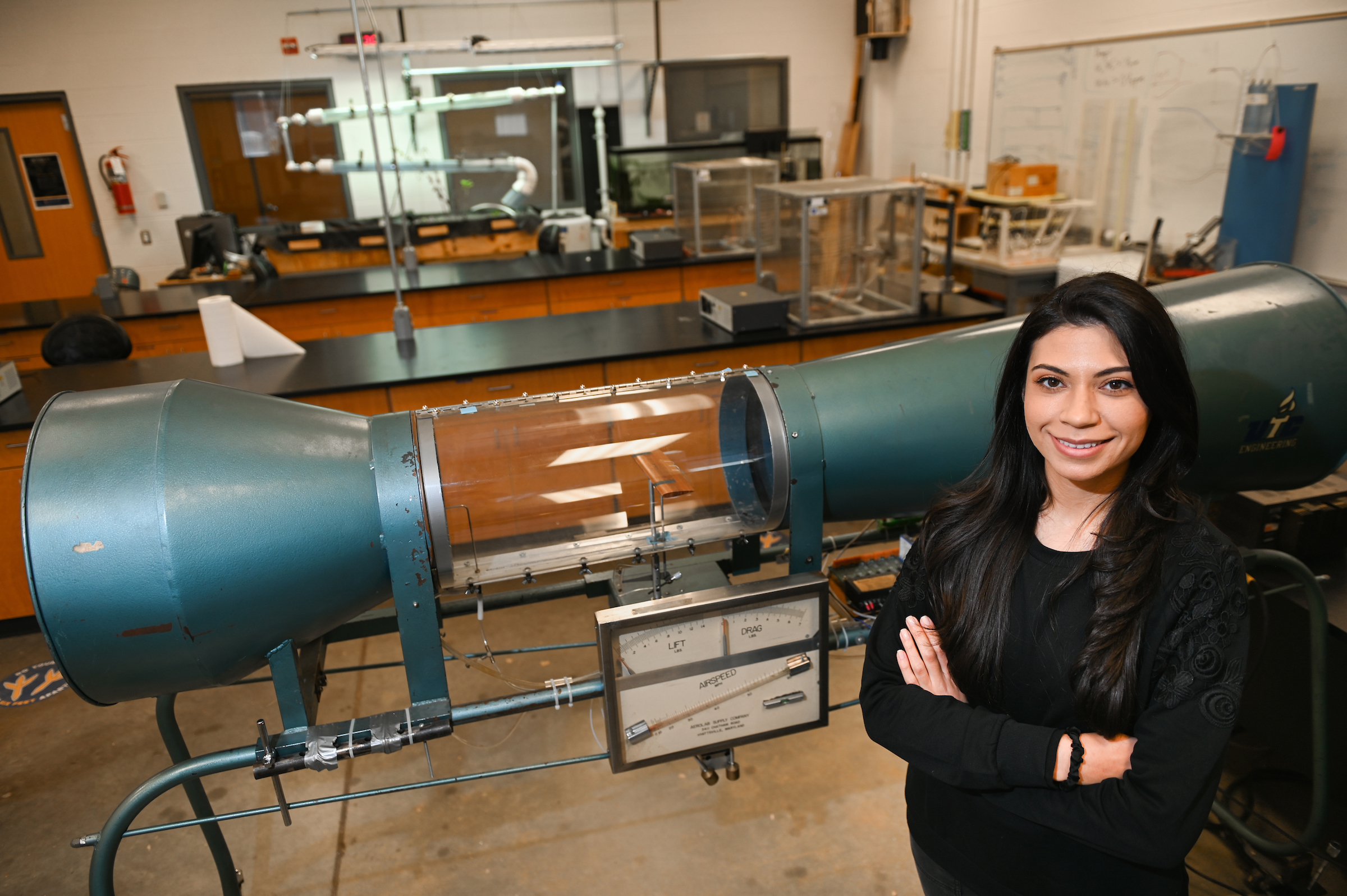
Trailblazing Arielle Scalioni building a civil engineering career

Posted on 5 May 2022 by Don Warrington

First-generation student Arielle Scalioni, a civil engineering major, will be receiving her bachelor’s degree from UTC during upcoming commencement ceremonies.

Source: Trailblazing Arielle Scalioni building a civil engineering career

Arielle was one of the smartest and most dedicated students I have ever had. It’s interesting that the main photo of her was in front the Wind Tunnel, which is part of my Fluid Mechanics Laboratory course. My prayers are with her as she pursues her career.

Academic Issues

We’re Where It’s At for Retaining Wall Books

Posted on 18 April 202217 April 2022 by Don Warrington

In the April/May 2022 issue of Geostrata, the chief publication of ASCE’s Geo-Institute, there is an article by Anne Lemnitzer and Eric Tavarez entitled “Earth Retaining Structure Design.” Among the results of the survey, an interesting one was the following:

The survey further asked universities what professional references are being introduced to students during their academic training on ERS. Among the available literature, the most heavily used were FHWA’s Geotechnical Engineering Circulars. Among the most selected circulars were:

GEC No. 2–Earth Retaining Systems
GEC No. 3–LRFD Seismic Analysis and Design of Transportation Geotechnical Features and Structural Foundations
GEC No. 4–Ground Anchors and Anchored Systems (also available in print)
GEC No. 7–Soil Nail Walls
GEC No. 11–Design and Construction of Mechanically Stabilized Earth Walls and Reinforced Soil Slopes (also available in print)

All but the first are in our collection (the first isn’t on the FHWA’s site either.) I have taking the liberty of noting that two of those are in print.

Even more gratifying is the following:

Several respondents used the open-response field to provide additional references they felt strongly about utilizing in the classroom. These included course materials for FHWA/NHI’s Soil and Foundations and Earth Retaining Structures courses (e.g., FHWA NHI-06-088, FHWA-NHI-132036, NHI-07-071, and the Army Corps of Engineers manuals and courses for the Design of Sheet Pile Walls (EM 1110-2-2504) and Tieback Wall Design and Construction (ERDC/ITL TR-02-011.)

Again most of these documents are on our site or on a companion site, free for download without restriction or login. Pride of place goes to the Soils and Foundations Reference Manual, which has been in print for a good while and which I use in my own Soil Mechanics and Foundation Design and Analysis courses.

A fairly new resource is my page on Vulcan and Sheet Piling, which deals with that subject in detail. And we have many other documents as well…

Since this site started twenty-five years ago this summer, there are many sources of information for this field, but we feel this one is unique.

Note: if you have the documents that are missing links above, and would like to have them on this site, get in touch with me and let's get it done.

Academic Issues

The Last Supper, the Iranians and the Perfect Dissertation: A Maundy Thursday Reflection

Posted on 14 April 202213 June 2024 by Don Warrington

In 2015 the PhD program I was going through nearly collapsed. We lost fifteen faculty members and key staff people in as many months. Needless to say, that produced consternation among the students, most of whom came from outside the United States. They did not understand our system (and honestly until I consulted with some officials of another university I didn’t either) required the University to support the program until the current students had graduated.

The exodus of faculty members created a great deal of empty office space. Like nature, bureaucracies abhor a vacuum, and my program director knew that, if he didn’t fill the office space, he would lose it. Since I was a faculty member (being faculty and student at the same time is as weird as it sounds) I got an office, the best one I ever had at UTC.

My office at UTC, where my Iranian colleagues admired the Last Supper sculpture on the top shelf.

One day one of my Iranian colleagues came to see me. She was going through the program with her husband. The two of them exuded the charm and sophistication that the Iranians are famous for. But she was drawn to the ceramic sculpture based on Leonardo da Vinci’s The Last Supper. It had been given to me when I was working for my church a decade earlier. You can see it in detail at the top of the post.

Not too long after that her husband came to see me. He too was drawn to the sculpture. I was amazed; the Iranians tended to be secular and this couple was from Isfahan, known for its own architecture.

We all eventually graduated and I retained the office for while. Eventually I was evicted; another Iranian colleague allowed me to split an office with him in another building, for which I was grateful because I was given no alternative. By then this person had become a Christian and had been baptized. In spite of the fact that yet another Iranian faculty colleague had assured me that this new building had “bad spirits” in it, we went forward.

But going back, to prepare for our dissertation defense, I attended a seminar where the Assistant Dean of the Graduate School, Dr. Randy Walker, assured us that he reviewed every dissertation and had never found one without a mistake. But our program director sent an email to all of us about my first office visitor:

I want to congratulate ________ for a first !!!! I received word from Dr. Randy Walker that __________’s dissertation was the first and only dissertation/thesis that he has reviewed that did not require any revisions.

Dr. Walker retired after this.

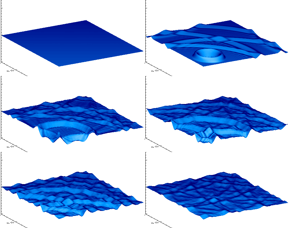
Results of the shallow water equation, the subject of the perfect dissertation.

A perfect dissertation at the end of the long effort a PhD is not common. But a perfect work is not unique. Maundy Thursday is the day in the Christian calendar when the Last Supper of Jesus Christ and his disciples is commemorated. Shortly after that, he was arrested by the authorities and crucified the following day. But on the following Sunday he rose from the dead.

Perfection was part of his being: “We have, then , in Jesus, the Son of God, a great High Priest who has passed into the highest Heaven; let us, therefore, hold fast to the Faith which we have professed. Our High Priest is not one unable to sympathize with our weaknesses, but one who has in every way been tempted, exactly as we have been, but without sinning.” (Hebrews 4:14-15 TCNT) His action on the cross was likewise complete: “…for then Christ would have had to undergo death many times since the creation of the world. But now, once and for all, at the close of the age, he has appeared, in order to abolish sin by the sacrifice of himself.” (Hebrews 9:26 TCNT)

Perfection and completeness are hard to obtain in this life. But if we make Jesus Christ’s work on the cross our own, we too can have them in this life and the next.

x/r	$\omega$
0	1.000	x/r	$\omega$
0.01	1.000	0.51	0.931
0.02	1.000	0.52	0.929
0.03	1.000	0.53	0.926
0.04	1.000	0.54	0.923
0.05	0.999	0.55	0.919
0.06	0.999	0.56	0.916
0.07	0.999	0.57	0.913
0.08	0.998	0.58	0.910
0.09	0.998	0.59	0.906
0.1	0.997	0.6	0.903
0.11	0.997	0.61	0.899
0.12	0.996	0.62	0.896
0.13	0.996	0.63	0.892
0.14	0.995	0.64	0.888
0.15	0.994	0.65	0.884
0.16	0.994	0.66	0.880
0.17	0.993	0.67	0.876
0.18	0.992	0.68	0.872
0.19	0.991	0.69	0.867
0.2	0.990	0.7	0.863
0.21	0.989	0.71	0.859
0.22	0.988	0.72	0.854
0.23	0.987	0.73	0.849
0.24	0.985	0.74	0.844
0.25	0.984	0.75	0.839
0.26	0.983	0.76	0.834
0.27	0.982	0.77	0.829
0.28	0.980	0.78	0.824
0.29	0.979	0.79	0.818
0.3	0.977	0.8	0.813
0.31	0.976	0.81	0.807
0.32	0.974	0.82	0.801
0.33	0.972	0.83	0.795
0.34	0.970	0.84	0.788
0.35	0.969	0.85	0.782
0.36	0.967	0.86	0.775
0.37	0.965	0.87	0.768
0.38	0.963	0.88	0.761
0.39	0.961	0.89	0.754
0.4	0.959	0.9	0.746
0.41	0.957	0.91	0.738
0.42	0.954	0.92	0.730
0.43	0.952	0.93	0.721
0.44	0.950	0.94	0.712
0.45	0.947	0.95	0.702
0.46	0.945	0.96	0.692
0.47	0.942	0.97	0.681
0.48	0.940	0.98	0.669
0.49	0.937	0.99	0.655
0.5	0.934	1	0.637

Circular Foundations

Foundations Rigid and Flexible

Other Sources

Share this:

Definitions (from Verruijt)

Assumptions

Theory of Elasticity of Infinite Strip Footings

Lower Bound Solution

Upper Bound

Worked Example

Conclusion

Share this:

Share this:

Share this:

For more information click here

Share this: