There’s a lot going on with this site, but one thing that needs some “catching up” is our marine construction collection, which really hasn’t received a comprehensive update since this site migrated to WordPress in 2016. We’ve added a number of documents to our collection: these are as follows (in no particular order): Coatings and […]
In a recent exchange Dr. Mark Svinkin, who has contributed several well-read articles to this site, pointed out that he had commented on a paper by Gazetas and Stokoe (1991.) The paper, Dr. Svinkin’s comments and their response can be found here:
Although this research was done a long time ago, it’s worth revisiting because of the issue that Dr. Svinkin brings up: the issue of size, that it’s not a straightforward business to extrapolate the results of model tests in controlled environments to full-scale foundations in actual stratigraphies.
In my fluid mechanics laboratory course, I discuss the issue of dynamic similarity, how one can take an airfoil or other flying object on a small scale and, using things such as the Reynolds Number, extrapolate those results to full-scale aircraft. This has proven very useful in the development of aircraft, especially before (and even long after) the development of simulation using computational fluid dynamics.
With geotechnical engineering, it has not been quite as simple. Attempts to use things such as centrifuge testing have not been as successful as, say, wind tunnel testing has been for aeronautics. Part of the problem is, as I like to say, that geotechinical engineering is not non-linear in the same sense as fluids are. Another problem is that the earth is not as homogeneous as the atmosphere, even when altitude and weather effects are considered (and these influence each other in the course of events.) But underneath all of this there are some fundamental issues that have complicated the issue of foundation size, and Dr. Svinkin points this out. My intent is to amplify on that and remind people that these issues are still relevant.
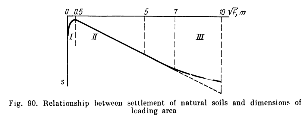
Dr. Svinkin points out the following figure from Tsytovich (1976.) I’ve referenced this text in several recent posts. Tsytovich looks at many problems in soil mechanics differently from our usual view in this country, and his perspective is frequently insightful. (An excellent example is here.) In this diagram he shows the effect of basic foundation size on the settlement of the foundation, and Tsytovich’s own explanation of this follows:
Relationship between settlement of natural soils and dimensions of loading area (from Tsytovich (1976).) The variable F is the area of the foundation, thus the square root of F is the basic dimension of the foundation and, in the case of square foundations, the exact dimension b or B (see below.)
Thus, Fig. 90 shows a generalized curve of the average results of numerous experiments on studying the settlements of earth bases (at an average degree of compaction) for the same pressure on soil but with different areas of loading. Three different regions may be distinguished on the curve: I —the region of small loading areas (approximately up to 0.25 m2) where soils at average pressures are predominantly in the shear phase, with the settlement being reduced with an increase of area (just opposite to what is predicted by the theory of elasticity for the phase of linear deformations); II — the region of areas from 0.25-0.50 m2 to 25-50 m2 (for homogeneous soils of medium density, and to higher values for weak soils), where settlements are strictly proportional to and at average pressures on soil correspond to the compaction phase, i.e., are very close to the theoretical ones; and III — the region of areas larger than 25-50 m2, where settlements are smaller than the theoretical ones, which may be explained by an increase of the soil modulus of elasticity (or a decrease of deform ability) with an increase of depth. For very loose and very dense soils these limits will naturally be somewhat different.
The data given can be used for establishing the limits of applicability of the theoretical solutions obtained for homogeneous massifs to real soils, which is of especial importance in developing rational methods of calculation of foundation settlements.
From Tsytovich (1976)
Although much of the discussion centred on Tsytovich and Barkan (1962,) there is evidence elsewhere to underscore this problem, which Tsytovich sets forth in a very succinct manner.
It is clear that, once one is past the basic soil properties and the pressure applied on the foundation, the settlement is proportional to the basic dimension of the foundation, which is exactly what is taking place in Region II. This is also why the bulk modulus of the soil is not a basic soil property, as I discuss in this lecture. When we consider plate load tests, we must correct them for the difference between the size of the test plate and the size of the foundation, as this slide presentation shows.
Since we are dealing with foundation dynamics, one item that seems to have fallen out of the whole discussion is that of Lysmer (1965). Lysmer’s Analogue, which reduces the response of a soil under the foundation to a simple spring-damper-mass system, defines the spring constant as follows:
(2)
where is the spring constant of the soil and is the foundation’s radius. If we break it down further, as is done in Warrington (1997,) and develop a unit area spring constant under the foundation, we have
(3)
where is the equivalent unit area spring constant under the soil. Equation (3) in particular shows that, for a given unit load on a foundation, the static portion of the reaction is inversely proportional to the basic size of the foundation. (The unit damping constant is actually independent of the area for round foundations.)
These results show that, while the effect of size may differ from one model to the next, it cannot be overlooked in any attempt to extrapolate physical model tests of any kind to actual use. This effect is further complicated by variations in shear modulus due to either strain softening, layered stratigraphy, effective stresses or other factors. The effect of the stratigraphy is further magnified by the fact that larger foundations have larger “bulbs of influence” into the soil and thus layers that smaller foundations would not interact with become significant with larger ones.
“Sand box” tests have other challenges. While they attempt to simulate a semi-infinite space, reflections from the walls of the box are inevitable, especially with periodic loads such as were present in this test. These challenges were documented in the original study. (An interesting study using another one of these boxes is that of Perry (1963).)
The failure of geotechnical engineering to adequately resolve the size issue, both in terms of design and in terms of using laboratory data to simulate full-scale performance, remains a frustration in geotechinical engineering. Hopefully other types of models will help move things forward, along with advances in our understanding of soil behaviour and our ability to replicate it both experimentally and numerically.
Next month, Lord willing, I start the second year of my PhD adventure in Computational Engineering. “Adventure” is a good way to describe it, especially in my superannuated state. In the midst of getting the coursework started last fall (yes, Europeans, sad to say we have coursework with PhD programmes) we had a “freshman” orientation.
One of the things my advisor oriented us about were the substantial computer capabilities that the SimCentre has. “Substantial” is a relative term; at one point we were in the top 500 computers in the world for power, but he chronicled our falling ranking which eventually left us “off the charts”. In spite of that the SimCentre continues to tout its capabilities and the rigour of its curriculum, and I can attest to the latter.
In my desperate attempt to re-activate brain cells long dormant (or activate a few that had never seen front-line service) I dug back and discovered that most of the “basics” of the trade were in place when I was an undergraduate in the 1970’s. Part of that process was discovering, for example, that one of the books I found most useful for projects like this had as a co-author one of my undergraduate professors! The biggest real change–and the one that drove just about everything else–was the rapid expansion of computer power from then until now. What has happened to the SimCentre was not that the computer cluster there had deteriorated; it has just not kept up with the ever-larger supercomputers coming on-line out there. Such is the challenge the institution faces.
One of my advisor’s favourite expressions is “in all its glory”, but in this case what we have is a case of “fading glory”. The SimCentre isn’t the only person or institution to face this problem:
If the system of religion which involved Death, embodied in a written Law and engraved on stones, began amid such glory, that the Israelites were unable to gaze at the face of Moses on account of its glory, though it was but a passing glory, Will not the religion that confers the Spirit have still greater glory? For, if there was a glory in the religion that involved condemnation, far greater is the glory of the religion that confers righteousness! Indeed, that which then had glory has lost its glory, because of the glory which surpasses it. And, if that which was to pass away was attended with glory, far more will that which is to endure be surrounded with glory! With such a hope as this, we speak with all plainness; Unlike Moses, who covered his face with a veil, to prevent the Israelites from gazing at the disappearance of what was passing away. (2 Corinthians 3:7-13)
When Moses came down from Mt. Sinai, having received the law directly from God (a truth that Muslims, along with Christians and Jews, affirm) he wore a veil:
Moses came down from Mount Sinai, carrying the two tablets with God’s words on them. His face was shining from speaking with the LORD, but he didn’t know it. When Aaron and all the Israelites looked at Moses and saw his face shining, they were afraid to come near him. Moses called to them, so Aaron and all the leaders of the community came back to him. Then Moses spoke to them. After that, all the other Israelites came near him, and he commanded them to do everything the LORD told him on Mount Sinai. When Moses finished speaking to them, he put a veil over his face. (Exodus 34:29-33)
Moses’ fellow Israelites were afraid to even come near him on account of the glory of God on his face, thus the veil. And Paul dutifully replicates this reasoning in 2 Corinthians 3:7. But Paul throws in another reason Moses needed to wear a veil: to hide the fact that, like the SimCentre’s computers, the glory was fading! That is what I call a “2 Corinthians 3” problem, and although Paul applies it to the Jewish law, it has broader application as well.
Today, in spite of our “flattened” society, we see people and institutions lifted up and presented as glorious. This is especially clear in the “messianic” streak that has entered our political life, but it’s also clear in the adulation given to celebrities, corporations and their products. It would behove us, however, to take a critical look at such things with one question: are we looking at real, enduring glory, or is this just another example of fading glory which is being covered up with hype?
As Paul and other New Testament authors note, the purpose of Jesus Christ coming to the earth was to solve the problem of fading glory, and specifically of a system that could not produce an entire solution to the problem of our sins and imperfections. Once that happens within ourselves, we can stop living behind the hype of whatever fading glory we’ve tried to hide behind and live in the truth.
‘Yet, whenever a man turns to the Lord, the veil is removed.’ And the ‘Lord’ is the Spirit, and, where the Spirit of the Lord is, there is freedom. And all of us, with faces from which the veil is lifted, seeing, as if reflected in a mirror, the glory of the Lord, are being transformed into his likeness, from glory to glory, as it is given by the Lord, the Spirit. (2 Corinthians 3:16-18)
It’s time to put a wrap on our series on constitutive equations, both elastic and plastic. We’ll do this in a more qualitative way by pointing out a trap in code writing that can have an effect on the results.
We generally divide problems into two kinds: static and dynamic. With static elastic problems, we can solve the equations in one shot, although we have to deal sometimes with geometric non-linearity (especially when elastic buckling is involved.) With dynamic problems time stepping is involved by definition. When we include plasticity, because of the path dependence issue we’re always using some kind of stepping in the solution. That stepping takes at least two levels: the stepping like we discussed in our last post and load and/or displacement stepping as the load or displacement is increased. Therefore, in a problem involving plasticity, we are stepping the problem one way or the other.
But how large do the steps need to be? In the case of dynamic stepping, that problem is wrapped up with the whole question of implicit vs. explicit methods. To make things simple, explicit methods are those which take information from the past and use that in each step to predict the state at the end of the step, while implicit methods use information from both start and finish of the step to predict the step end state. Implicit methods have the advantage of allowing the model to have larger time steps, which is one reason why they’ve gained currency with, say, computational fluid dynamics models.
It would seem that using an implicit method would be the optimal solution for a dynamic system. However, that runs into a serious problem, as discussed by Warrington (2016):
Consider the elasto-plastic model as depicted (above). At low values of strain, elasticity applies and the relationship between stress and strain is determined by the slope of the line, the modulus of elasticity. In the elasto-plastic models considered, the reality is that the relationship between stress and strain is always linear; the key difference between the elastic and plastic regions is that, upon entrance into the plastic region, there are irrecoverable strains which take place. Cook, Malkus and Plesha (1989) observe that, in the plastic region, there is a plastic modulus, which is less than the elastic modulus and, in the case of softening materials, actually negative. They also observe that, in this region, the acoustic speed is lower than that in the elastic region…This is a similar phenomenon to that of the variations in elastic modulus and acoustic speed based on strain, which complicated the determination of the applicable soil properties.
With a purely elasto-plastic model, the plastic modulus is zero, and thus the acoustic speed is also zero. This effectively decouples the mass from the elasticity in the purely plastic region. This result is more pronounced as the time (and thus the distance) step is increased; the model tends to “skip over” the elastic region and the inertial effects in that region. Thus with larger time steps inertial effects are significantly reduced, and their ability to resist pile movement is likewise reduced.
For problems such as this, the best solution is to use an explicit method with very small time steps to “catch” all of the effects of the plasticity. One major advantage of that approach is that explicit methods allow us to dispense with assembling the global stiffness matrix, giving rise to “matrix-free” methods you hear about. That significantly reduces both memory requirements and computational costs in a model. It has also led to changing even problems we consider as “static” (like static load testing) to dynamic problems with small time steps, no stiffness matrices and long run times, an acknowledgement that, strictly speaking, there are no real “static” problems, a fact that makes many civil engineers freak out.
Chances are that the effects of this have been built into whatever code you might be using, and that you’re not aware of how your code is handing it. The wise user of numerical modelling solutions would do well to familiarise him or herself of how the code being used actually handles problems such as this and becomes a more informed user of the tools at hand.
With the Mohr-Coulomb failure criterion defined, the elasto-plastic constitutive matrix can be developed. Since pure plasticity is assumed, thus once failure is reached and F=0 , the stresses can “rearrange” themselves to remain at the failure surface but cannot move from it unless the strains are reduced to the point where the stress state is within the failure surface and F<0. This is easier to see if we look at the diagram above. We should also note that, for this presentation, the plane strain/axisymmetric case will be considered; the derivation would proceed a little differently for other cases such as plane stress or three-dimensional stress.
To do this, both Equations 8 and 10 from the previous post are differentiated. Considering that
(1)
for the two-dimensional model, then
(2)
where
(3)
and
(4)
Inspection of Equation 3 will show that C2 and C3 are undefined for values of θ =30°. This is the well known “corner” problem which has occupied the literature for many years, as summarized by Abbo et.al. (2011). For this study the “corner cutting” of Owen and Hinton (1980) is used, and
(5)
Although the accuracy of this “corner cutting” can be improved with methods such as those of Abbo et.al. (2011), they come at more computational expense.
In like fashion for the plastic potential function,
(6)
where
(7)
and by extension
(8)
and the vectors a1 , a2 , a3are the same as with Equation 2.
At this point we need to pause and consider how we plan to present our result. It’s certain possible, for example, to multiply through Equations 2, 3, and 4 and use this result in subsequent derivations. This approach suffers from two problems: the element expressions in the matrices and vectors become very complicated, and the computation cost is increased by the repetitive calculations. For some good advice on this subject–for this and other problems–we would suggest that you review this.
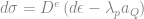
Now the elasto-plastic constitutive matrix can be considered. Here the difference between path indepedence and path dependence becomes significant. In the elastic case, we can use the elastic consitutive matrix De and, knowing the strains, compute the stresses, and perform the inverse as well. With plasticity, it is necessary to compute the strains and stresses incrementally, moving from one stress and strain state to the next and adding the results to what has gone before. We do this with both elastic, plastic and combined strains and stresses for computational consistency. The elastic results will be the same except for the additional accumulation of numerical error due to the larger number of computations.
For any strain increment partially or totally beyond the yield surface, that strain increment will contain both elastic and plastic portions (Griffiths and Willson (1986)), or
(9)
Strain increments occur normal to the plastic potential surface, thus
(10)
For elastic materials, the incremental stress-strain relationship is simply
(11)
where, for plane strain and axisymmetric problems, as before,
(12)
and also, for axisymmetric problems only,
(13)
For a perfectly elasto-plastic material, i.e., one without hardening or softening, stress changes will take place only during elastic action. Thus in these cases Equations 9, 10 and 11 can be rearranged to yield
(14)
Since stresses on the failure surface can “rearrange” themselves without leaving same surface,
(15)
Combining and rearranging Equations 9 through 15 yields the following relationships:
(16)
(17)
or
(18)
where
(19)
and finally
(20)
We need to break this down for greater understanding. Let us first define
(21)
This is a scalar quantity. (Admittedly sometimes it is difficult to follow matrix equations because they combine scalar and vector/matrix quantities.) We can thus rewrite Equation 19
(22)
and Equation 20 can be likewise rewritten as
(23)
where the identity matrix.
If plasticity has not yet been initiated, the quantity (which is a 4 x 4 matrix) is null, and the elasticity matrix governs. Once it is initiated the magnitude of begins to increase and Dep begins to decrease, which indicates a ‘softening’ of the material. This is what we would expect with plasticity. The whole topic of matrix magnitude is not a straightforward one and is usually viewed in relationship to matrix norms, which are discussed in Gourdin and Boumharat (1989).
In any case
(24)
The first thing to note about Equation 20 is that, if same is used to reconstruct a tangent stiffness matrix KT in a true Newton stepping scheme, same KT will not be symmetric if φ ≠ ψ. For many engineering materials, and especially those where both of these quantities are zero, this is not an issue; the flow rule is associated, Dep is symmetric and KT will be also. “Regular” engineering materials are used for, say, the steel or concrete portions of a system, but for many geotechincal applications interest in plastic deformation of these components is limited. It is also not an issue with purely cohesive soils. For situations with cohesionless soils, this is not the case; generally φ ≫ ψ and a non-associated flow rule is necessary. This aspect will be important in many decisions regarding the structure and types of schemes used in the model. An overview of the values of the dilitancy angle ψ can be found in Warrington (2019).
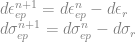
Turning to the inclusion of plasticity itself, it is certainly possible to compute the plastic stresses from Equation 20, and also possible to explicitly derive Equation 19 (Griffiths and Willson (1986)). However, it is not always optimal to do so, either from the standpoint of a workable algorithm or from a computational efficiency standpoint. To compute the final stress state in a load or time step where failure takes place, some type of iteration or multiple steps are required. Potts and Zdravkovic (1999) state that there are two basic types of algorithms to accomplish this: substepping (such as Sloan (1987)) and return (Ortiz and Simo (1986)). For STADYN a return algorithm was chosen, and implemented as follows:
For a load or time step, the estimated incremental strain was computed.
The estimated incremental stress was computed, based on the assumption that the strains were still in the elastic region.
The resulting incremental stresses were added to the stresses at the beginning of the step. If these were elastic, then plasticity was not considered and the incremental stresses were added to the original ones. If they were not, then the plasticity routine was invoked.
The plasticity routine began by computing aF , aQ , F , θ and aβ.
The plasticity constant λp was determined by a modification to Equation 16, namely (25)
The incremental strains in the return step were computed by the equation (see Equation 14) (26)
The return incremental stresses were thus (27)
Both of these were subtracted from the current estimated strain and stress, thus (28)
The current stress state was checked against the previous stress state. If the norm of the vector difference of the two stress states was within the convergence tolerance, the iteration was stopped and the computed elasto-plastic stresses and strains were accepted. If not, the cycle was repeated.
Potts and Zdravkovic (1999) criticize the return algorithms because they obtain a result based on information and computations in illegal stress space. However, overall the experience in this study is that the return algorithm worked well, with most of the convergence to the new failure surface stress state taking place in the first iteration and the rest refinement steps. A fair way of differentiating between the two is that, with substepping, one starts with the existing stress state and works one’s way to the failure surface, while the return algorithm starts by overshooting the failure surface and then coming back to it. The goal in both cases is to return to the failure surface, and in principle the result should be the same. Another way of differentiating between the two is that substepping is, with its avoidance of illegal stresses, more of an engineering type of approach to the problem, while the return algorithm is a more strictly mathematical method of arriving at a solution.


 and at average pressures on soil correspond to the compaction phase, i.e., are very close to the theoretical ones; and III — the region of areas larger than 25-50 m2, where settlements are smaller than the theoretical ones, which may be explained by an increase of the soil modulus of elasticity (or a decrease of deform ability) with an increase of depth. For very loose and very dense soils these limits will naturally be somewhat different.
 (1)
(1) settlement of the foundation at the point of interest
 influence factor, given in the table below
 uniform pressure on the foundation
 smaller dimension of rectangle or dimension of square side
 Poisson’s Ratio of the soil
 Modulus of elasticity of the soil
 are shown below.
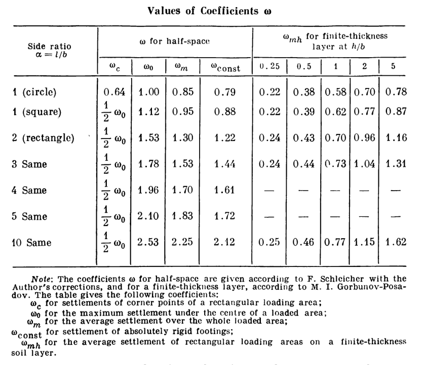
 (2)
(2) is the spring constant of the soil and
  is the foundation’s radius. If we break it down further, as is done in
  (3)
(3) is the equivalent unit area spring constant under the soil. Equation (3) in particular shows that, for a given unit load on a foundation, the static portion of the reaction is inversely proportional to the basic size of the foundation. (The unit damping constant is actually independent of the area for round foundations.)
![\sigma=\left[\begin{array}{c} \sigma_{x}\\ \sigma_{y}\\ \sigma_{z}\\ \tau_{xy} \end{array}\right]](https://s0.wp.com/latex.php?latex=%5Csigma%3D%5Cleft%5B%5Cbegin%7Barray%7D%7Bc%7D+%5Csigma_%7Bx%7D%5C%5C+%5Csigma_%7By%7D%5C%5C+%5Csigma_%7Bz%7D%5C%5C+%5Ctau_%7Bxy%7D+%5Cend%7Barray%7D%5Cright%5D+&bg=ffffff&fg=777777&s=0&c=20201002) (1)
(1) (2)
(2)
![C_{2}=cos\theta\left[\left(1+tan\theta tan3\theta\right)+\frac{sin\phi\left(tan3\theta-tan\theta\right)}{\sqrt{3}}\right]](https://s0.wp.com/latex.php?latex=C_%7B2%7D%3Dcos%5Ctheta%5Cleft%5B%5Cleft%281%2Btan%5Ctheta+tan3%5Ctheta%5Cright%29%2B%5Cfrac%7Bsin%5Cphi%5Cleft%28tan3%5Ctheta-tan%5Ctheta%5Cright%29%7D%7B%5Csqrt%7B3%7D%7D%5Cright%5D+&bg=ffffff&fg=777777&s=0&c=20201002) (3)
(3)
![a_{1}=\left[\begin{array}{c} 1\\ 1\\ 1\\ 0 \end{array}\right]](https://s0.wp.com/latex.php?latex=a_%7B1%7D%3D%5Cleft%5B%5Cbegin%7Barray%7D%7Bc%7D+1%5C%5C+1%5C%5C+1%5C%5C+0+%5Cend%7Barray%7D%5Cright%5D+&bg=ffffff&fg=777777&s=0&c=20201002)
![a_{2}=\frac{1}{2\sqrt{J'_{2}}}\left[\begin{array}{c} \sigma'_{x}\\ \sigma'_{y}\\ \sigma'_{z}\\ 2\tau_{xy} \end{array}\right]](https://s0.wp.com/latex.php?latex=a_%7B2%7D%3D%5Cfrac%7B1%7D%7B2%5Csqrt%7BJ%27_%7B2%7D%7D%7D%5Cleft%5B%5Cbegin%7Barray%7D%7Bc%7D+%5Csigma%27_%7Bx%7D%5C%5C+%5Csigma%27_%7By%7D%5C%5C+%5Csigma%27_%7Bz%7D%5C%5C+2%5Ctau_%7Bxy%7D+%5Cend%7Barray%7D%5Cright%5D+&bg=ffffff&fg=777777&s=0&c=20201002) (4)
(4)![a_{3}=\left[\begin{array}{c} \sigma'_{y}\sigma'_{z}+\frac{J'_{2}}{3}\\ \sigma'_{x}\sigma'_{z}+\frac{J'_{2}}{3}\\ \sigma'_{y}\sigma'_{x}-\tau_{xy}^{2}+\frac{J'_{2}}{3}\\ -2\sigma'_{z}\tau_{xy} \end{array}\right]](https://s0.wp.com/latex.php?latex=a_%7B3%7D%3D%5Cleft%5B%5Cbegin%7Barray%7D%7Bc%7D+%5Csigma%27_%7By%7D%5Csigma%27_%7Bz%7D%2B%5Cfrac%7BJ%27_%7B2%7D%7D%7B3%7D%5C%5C+%5Csigma%27_%7Bx%7D%5Csigma%27_%7Bz%7D%2B%5Cfrac%7BJ%27_%7B2%7D%7D%7B3%7D%5C%5C+%5Csigma%27_%7By%7D%5Csigma%27_%7Bx%7D-%5Ctau_%7Bxy%7D%5E%7B2%7D%2B%5Cfrac%7BJ%27_%7B2%7D%7D%7B3%7D%5C%5C+-2%5Csigma%27_%7Bz%7D%5Ctau_%7Bxy%7D+%5Cend%7Barray%7D%5Cright%5D+&bg=ffffff&fg=777777&s=0&c=20201002)
![C_{2}=\frac{1}{2}\left[\sqrt{3}-\frac{sin\phi}{\sqrt{3}}\right],\:\theta\approx\pm30^{\circ}](https://s0.wp.com/latex.php?latex=C_%7B2%7D%3D%5Cfrac%7B1%7D%7B2%7D%5Cleft%5B%5Csqrt%7B3%7D-%5Cfrac%7Bsin%5Cphi%7D%7B%5Csqrt%7B3%7D%7D%5Cright%5D%2C%5C%3A%5Ctheta%5Capprox%5Cpm30%5E%7B%5Ccirc%7D+&bg=ffffff&fg=777777&s=0&c=20201002) (5)
(5)
 (6)
(6)![C_{4}=\frac{sin\psi}{3}\\C_{5}=cos\theta\left[\left(1+tan\theta tan3\theta\right)+\frac{sin\psi\left(tan3\theta-tan\theta\right)}{\sqrt{3}}\right]\\C_{6}=\frac{\sqrt{3}sin\theta+cos\theta sin\psi}{2J'_{2}cos3\theta}](https://s0.wp.com/latex.php?latex=C_%7B4%7D%3D%5Cfrac%7Bsin%5Cpsi%7D%7B3%7D%5C%5CC_%7B5%7D%3Dcos%5Ctheta%5Cleft%5B%5Cleft%281%2Btan%5Ctheta+tan3%5Ctheta%5Cright%29%2B%5Cfrac%7Bsin%5Cpsi%5Cleft%28tan3%5Ctheta-tan%5Ctheta%5Cright%29%7D%7B%5Csqrt%7B3%7D%7D%5Cright%5D%5C%5CC_%7B6%7D%3D%5Cfrac%7B%5Csqrt%7B3%7Dsin%5Ctheta%2Bcos%5Ctheta+sin%5Cpsi%7D%7B2J%27_%7B2%7Dcos3%5Ctheta%7D+&bg=ffffff&fg=777777&s=0&c=20201002) (7)
(7)![C_{4}=\frac{sin\psi}{3}\\C_{5}=\frac{1}{2}\left[\sqrt{3}-\frac{sin\psi}{\sqrt{3}}\right],\:\theta\approx\pm30^{\circ}\\C_{6}=0](https://s0.wp.com/latex.php?latex=C_%7B4%7D%3D%5Cfrac%7Bsin%5Cpsi%7D%7B3%7D%5C%5CC_%7B5%7D%3D%5Cfrac%7B1%7D%7B2%7D%5Cleft%5B%5Csqrt%7B3%7D-%5Cfrac%7Bsin%5Cpsi%7D%7B%5Csqrt%7B3%7D%7D%5Cright%5D%2C%5C%3A%5Ctheta%5Capprox%5Cpm30%5E%7B%5Ccirc%7D%5C%5CC_%7B6%7D%3D0+&bg=ffffff&fg=777777&s=0&c=20201002) (8)
(8) (9)
(9) (10)
(10) (11)
(11)![D^{e}=\left[\begin{array}{cccc} {\frac{\left(1-\nu\right)\lambda}{\nu}} & \lambda & \lambda & 0\\ \noalign{\medskip}\lambda & {\frac{\left(1-\nu\right)\lambda}{\nu}} & \lambda & 0\\ \noalign{\medskip}\lambda & \lambda & {\frac{\left(1-\nu\right)\lambda}{\nu}} & 0\\ \noalign{\medskip}0 & 0 & 0 & G \end{array}\right]](https://s0.wp.com/latex.php?latex=D%5E%7Be%7D%3D%5Cleft%5B%5Cbegin%7Barray%7D%7Bcccc%7D+%7B%5Cfrac%7B%5Cleft%281-%5Cnu%5Cright%29%5Clambda%7D%7B%5Cnu%7D%7D+%26+%5Clambda+%26+%5Clambda+%26+0%5C%5C+%5Cnoalign%7B%5Cmedskip%7D%5Clambda+%26+%7B%5Cfrac%7B%5Cleft%281-%5Cnu%5Cright%29%5Clambda%7D%7B%5Cnu%7D%7D+%26+%5Clambda+%26+0%5C%5C+%5Cnoalign%7B%5Cmedskip%7D%5Clambda+%26+%5Clambda+%26+%7B%5Cfrac%7B%5Cleft%281-%5Cnu%5Cright%29%5Clambda%7D%7B%5Cnu%7D%7D+%26+0%5C%5C+%5Cnoalign%7B%5Cmedskip%7D0+%26+0+%26+0+%26+G+%5Cend%7Barray%7D%5Cright%5D+&bg=ffffff&fg=777777&s=0&c=20201002) (12)
(12)![\epsilon^{e}=\left[\begin{array}{c} \epsilon_{r}\\ \epsilon_{z}\\ \epsilon_{\theta}\\ \epsilon_{rz} \end{array}\right]](https://s0.wp.com/latex.php?latex=%5Cepsilon%5E%7Be%7D%3D%5Cleft%5B%5Cbegin%7Barray%7D%7Bc%7D+%5Cepsilon_%7Br%7D%5C%5C+%5Cepsilon_%7Bz%7D%5C%5C+%5Cepsilon_%7B%5Ctheta%7D%5C%5C+%5Cepsilon_%7Brz%7D+%5Cend%7Barray%7D%5Cright%5D+&bg=ffffff&fg=777777&s=0&c=20201002) (13)
(13) (14)
(14) (15)
(15) (16)
(16) (17)
(17) (18)
(18) (19)
(19) (20)
(20) (21)
(21) (22)
(22) (23)
(23) the identity matrix.
 (which is a 4 x 4 matrix) is null, and the elasticity matrix governs. Once it is initiated the magnitude of
  (24)
(24) (25)
(25) (26)
(26) (27)
(27) (28)
(28)