Constitutive Elasticity Equations: Three-Dimensional Formulation

This is the beginning of what hopefully will be an enlightening series on elasticity and plasticity, primarily as it appears in finite element code. It is taken from a number of sources, including (but not limited to) Owen and Hinton (1980), Smith and Griffiths (1988) and Cook, Malkus and Plesha (1989.) Although finite element code has certainly advanced, the basics are still the same, especially with elasticity (plasticity is another matter.) More information on finite element analysis in geotechnics (with a link to Owen and Hinton) can be found here.

The basic elasticity relationship is familiar to engineers and can be stated as follows:

$\sigma = E \epsilon$ (1)

where

$\sigma =$ stress
$E =$ Young’s modulus, or modulus of elasticity
$\epsilon =$ strain

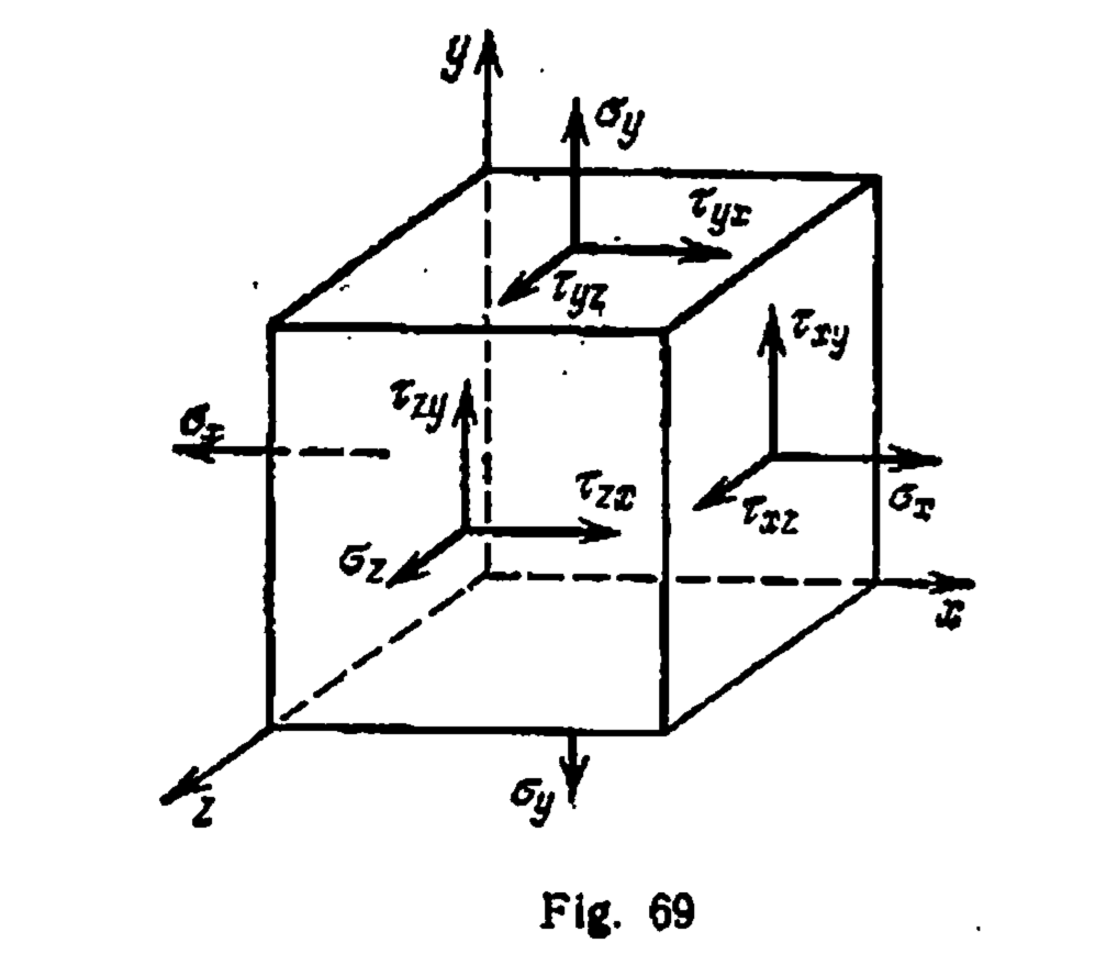
Element with normal and shear stresses (from Belyaev (1979))

It can be used in one-dimensional analyses such as tension and compression testing; we’ll come back to that later. But real problems are always in three dimensions in one way or another. Let’s start by considering an infinitesimal element (these are discussed in Verruijt) that looks like the one in Figure 69. There are many ways of looking at this element. For one thing, it is in static equilibrium, which means that the stresses can be changed along with the coordinate system and the results still be in static equilibrium. Related to this is the fact that there is one coordinate system at which point the shear stresses vanish and the three normal stresses that are left are the principal stresses; this is discussed here.

These, however, are not our main interest here. Our main interest is how the element deforms under stress. For now we will restrict our discussion to elastic, path-independent stresses. We will rewrite Equation (1) is a slightly different form:

$D \epsilon = \sigma$ (2)

Now both $\sigma$ and $\epsilon$ are vectors; you can see the multiple stresses in Figure 69. We use the notation $D$ because the modulus of elasticity $E$ is a material property and thus is a part of the elasticity matrix $D$ .

In any case, when the actual vector and matrices are substituted into Equation (2), for three-dimensional problems such as shown in Figure 69 the equations look like this:

$\left[\begin{array}{cccccc} {\frac{{\it E}\,\left(1-\nu\right)}{\left(1+\nu\right)\left(1-2\,\nu\right)}} & {\frac{{\it E}\,\nu}{\left(1+\nu\right)\left(1-2\,\nu\right)}} & {\frac{{\it E}\,\nu}{\left(1+\nu\right)\left(1-2\,\nu\right)}} & 0 & 0 & 0\\ \noalign{\medskip}{\frac{{\it E}\,\nu}{\left(1+\nu\right)\left(1-2\,\nu\right)}} & {\frac{{\it E}\,\left(1-\nu\right)}{\left(1+\nu\right)\left(1-2\,\nu\right)}} & {\frac{{\it E}\,\nu}{\left(1+\nu\right)\left(1-2\,\nu\right)}} & 0 & 0 & 0\\ \noalign{\medskip}{\frac{{\it E}\,\nu}{\left(1+\nu\right)\left(1-2\,\nu\right)}} & {\frac{{\it E}\,\nu}{\left(1+\nu\right)\left(1-2\,\nu\right)}} & {\frac{{\it E}\,\left(1-\nu\right)}{\left(1+\nu\right)\left(1-2\,\nu\right)}} & 0 & 0 & 0\\ \noalign{\medskip}0 & 0 & 0 & {\frac{{\it E}\,\left(1-\nu\right)}{\left(1+\nu\right)\left(2-2\,\nu\right)}} & 0 & 0\\ \noalign{\medskip}0 & 0 & 0 & 0 & {\frac{{\it E}\,\left(1-\nu\right)}{\left(1+\nu\right)\left(2-2\,\nu\right)}} & 0\\ \noalign{\medskip}0 & 0 & 0 & 0 & 0 & {\frac{{\it E}\,\left(1-\nu\right)}{\left(1+\nu\right)\left(2-2\,\nu\right)}} \end{array}\right]\left[\begin{array}{c} \epsilon_{{x}}\\ \noalign{\medskip}\epsilon_{{y}}\\ \noalign{\medskip}\epsilon_{{z}}\\ \noalign{\medskip}\gamma{}_{{\it xy}}\\ \noalign{\medskip}{\it \gamma}_{{\it yz}}\\ \noalign{\medskip}{\it \gamma}_{{\it zx}} \end{array}\right]=\left[\begin{array}{c} \sigma_{{x}}\\ \noalign{\medskip}\sigma_{{y}}\\ \noalign{\medskip}\sigma_{{z}}\\ \noalign{\medskip}\tau_{{\it xy}}\\ \noalign{\medskip}\tau_{{\it yz}}\\ \noalign{\medskip}\tau_{{\it zx}} \end{array}\right]$ (3)

It should be immediately apparent that there are many repetitious quantities. There are many ways of dealing with the problem. For this analysis we will substitute Lamé’s constants, which are

$\lambda = \frac{\nu E}{(1+\nu)(1-2\nu)}$ (4)

$G = \frac{E}{2(1+\nu)}$ (5)

where $\nu$ is Poisson’s Ratio and $G$ is the shear modulus of elasticity. The latter is very useful in soil mechanics (which can be seen, for example, here) and in fact Equation (4) can be restated as follows:

$\lambda = \frac{2\nu G}{1-2\nu}$ (6)

At this point we need to observe one important thing: no matter whether you use Equation (4) or (6), the Lamé constant $\lambda$ blows up (or becomes singular, as we say in polite circles) when $\nu = \frac{1}{2}$ . Materials where this is the case (such as very soft clays) are in reality fluids, the normal stresses become equal and the shear stresses only appear when the fluid moves. Avoiding this condition is one of the challenges of geotechnical finite element analysis.

It’s also worth noting that this is the same Lamé who came up with the theory behind shrink fits that is important with Vulcan hammers.

In any case, if we apply Equations (5) and (4) or (6), we obtain the following:

$\left[\begin{array}{cccccc} {\frac{\left(1-\nu\right)\lambda}{\nu}} & \lambda & \lambda & 0 & 0 & 0\\ \noalign{\medskip}\lambda & {\frac{\left(1-\nu\right)\lambda}{\nu}} & \lambda & 0 & 0 & 0\\ \noalign{\medskip}\lambda & \lambda & {\frac{\left(1-\nu\right)\lambda}{\nu}} & 0 & 0 & 0\\ \noalign{\medskip}0 & 0 & 0 & G & 0 & 0\\ \noalign{\medskip}0 & 0 & 0 & 0 & G & 0\\ \noalign{\medskip}0 & 0 & 0 & 0 & 0 & G \end{array}\right] \left[\begin{array}{c} \epsilon_{{x}}\\ \noalign{\medskip}\epsilon_{{y}}\\ \noalign{\medskip}\epsilon_{{z}}\\ \noalign{\medskip}\gamma{}_{{\it xy}}\\ \noalign{\medskip}{\it \gamma}_{{\it yz}}\\ \noalign{\medskip}{\it \gamma}_{{\it zx}} \end{array}\right]=\left[\begin{array}{c} \sigma_{{x}}\\ \noalign{\medskip}\sigma_{{y}}\\ \noalign{\medskip}\sigma_{{z}}\\ \noalign{\medskip}\tau_{{\it xy}}\\ \noalign{\medskip}\tau_{{\it yz}}\\ \noalign{\medskip}\tau_{{\it zx}} \end{array}\right]$ (7)

We see from this that we have simplified assembling the constitutive matrix considerably. From a coding standpoint, doing this eliminates not only the possibility of coding error but also computational cost by eliminating the sheer number of operations. This is especially useful if these matrices are reconstituted during the analysis (as one would expect if strain-softening is applied, for example.)

If we multiply the left hand side through, we have

$\left[\begin{array}{c} \sigma_{{x}}\\ \noalign{\medskip}\sigma_{{y}}\\ \noalign{\medskip}\sigma_{{z}}\\ \noalign{\medskip}\tau_{{\it xy}}\\ \noalign{\medskip}\tau_{{\it yz}}\\ \noalign{\medskip}\tau_{{\it zx}} \end{array}\right] = \left[\begin{array}{c} {\frac{\left(1-\nu\right)\lambda\,\epsilon_{{x}}}{\nu}}+\lambda\,\epsilon_{{y}}+\lambda\,\epsilon_{{z}}\\ \noalign{\medskip}\lambda\,\epsilon_{{x}}+{\frac{\left(1-\nu\right)\lambda\,\epsilon_{{y}}}{\nu}}+\lambda\,\epsilon_{{z}}\\ \noalign{\medskip}\lambda\,\epsilon_{{x}}+\lambda\,\epsilon_{{y}}+{\frac{\left(1-\nu\right)\lambda\,\epsilon_{{z}}}{\nu}}\\ \noalign{\medskip}G{\it \gamma}_{{\it xy}}\\ \noalign{\medskip}G{\it \gamma}_{{\it yz}}\\ \noalign{\medskip}G{\it \gamma}_{{\it zx}} \end{array}\right]$ (8)

Inversely, if we want to know the strains, we would compute these by the relationship

$\epsilon = D^{-1} \sigma$ (9)

Inverting,

$D_{e}^{-1}=\left[\begin{array}{cccccc} -{\frac{\nu}{\lambda\,\left(-1+\nu+2\,{\nu}^{2}\right)}} & {\frac{{\nu}^{2}}{\lambda\,\left(-1+\nu+2\,{\nu}^{2}\right)}} & {\frac{{\nu}^{2}}{\lambda\,\left(-1+\nu+2\,{\nu}^{2}\right)}} & 0 & 0 & 0\\ \noalign{\medskip}{\frac{{\nu}^{2}}{\lambda\,\left(-1+\nu+2\,{\nu}^{2}\right)}} & -{\frac{\nu}{\lambda\,\left(-1+\nu+2\,{\nu}^{2}\right)}} & {\frac{{\nu}^{2}}{\lambda\,\left(-1+\nu+2\,{\nu}^{2}\right)}} & 0 & 0 & 0\\ \noalign{\medskip}{\frac{{\nu}^{2}}{\lambda\,\left(-1+\nu+2\,{\nu}^{2}\right)}} & {\frac{{\nu}^{2}}{\lambda\,\left(-1+\nu+2\,{\nu}^{2}\right)}} & -{\frac{\nu}{\lambda\,\left(-1+\nu+2\,{\nu}^{2}\right)}} & 0 & 0 & 0\\ \noalign{\medskip}0 & 0 & 0 & {G}^{-1} & 0 & 0\\ \noalign{\medskip}0 & 0 & 0 & 0 & {G}^{-1} & 0\\ \noalign{\medskip}0 & 0 & 0 & 0 & 0 & {G}^{-1} \end{array}\right]$ (10)

and the strains can be computed as follows

$\left[\begin{array}{c} \epsilon_{{x}}\\ \noalign{\medskip}\epsilon_{{y}}\\ \noalign{\medskip}\epsilon_{{z}}\\ \noalign{\medskip}\gamma{}_{{\it xy}}\\ \noalign{\medskip}{\it \gamma}_{{\it yz}}\\ \noalign{\medskip}{\it \gamma}_{{\it zx}} \end{array}\right] = \left[\begin{array}{c} -{\frac{\nu\,\sigma_{{x}}}{\lambda\,\left(-1+\nu+2\,{\nu}^{2}\right)}}+{\frac{{\nu}^{2}\sigma_{{y}}}{\lambda\,\left(-1+\nu+2\,{\nu}^{2}\right)}}+{\frac{{\nu}^{2}\sigma_{{z}}}{\lambda\,\left(-1+\nu+2\,{\nu}^{2}\right)}}\\ \noalign{\medskip}{\frac{{\nu}^{2}\sigma_{{x}}}{\lambda\,\left(-1+\nu+2\,{\nu}^{2}\right)}}-{\frac{\nu\,\sigma_{{y}}}{\lambda\,\left(-1+\nu+2\,{\nu}^{2}\right)}}+{\frac{{\nu}^{2}\sigma_{{z}}}{\lambda\,\left(-1+\nu+2\,{\nu}^{2}\right)}}\\ \noalign{\medskip}{\frac{{\nu}^{2}\sigma_{{x}}}{\lambda\,\left(-1+\nu+2\,{\nu}^{2}\right)}}+{\frac{{\nu}^{2}\sigma_{{y}}}{\lambda\,\left(-1+\nu+2\,{\nu}^{2}\right)}}-{\frac{\nu\,\sigma_{{z}}}{\lambda\,\left(-1+\nu+2\,{\nu}^{2}\right)}}\\ \noalign{\medskip}{\frac{\tau_{{\it xy}}}{G}}\\ \noalign{\medskip}{\frac{\tau_{{\it yz}}}{G}}\\ \noalign{\medskip}{\frac{\tau_{{\it zx}}}{G}} \end{array}\right]$ (11)

Relationships such as Equations (8) and (11) will be more useful when we consider two-dimensional problems.

References

Cook, R.D., Malkus, D.S. and Plesha, M.E. (1989). Concepts and Applications of Finite Element Analysis, John Wiley & Sons, Inc., New York, NY
Owen, D.R.J., and Hinton, E. (1980). Finite Elements in Plasticity: Theory and Practice. Pineridge Press, Swansea, Wales.
Smith, I.M., and Griffiths, D.V. (1988). Programming the Finite Element Method. Second Edition. John Wiley & Sons, Chichester, England.

Note: after this was first posted, some errors were discovered. These were corrected with the assistance of Jaeger, J.C. and Cook, N.G.W. (1979) Fundamentals of Rock Mechanics. London: Chapman and Hall. This book has an excellent treatment of basic theoretical solid mechanics in general and elasticity in particular. Although they do not put the equations in matrix form, they do use the Lamé constants in their formulation, albeit in a different way than is done here. We apologise for any inconvenience or confusion.

10 thoughts on “Constitutive Elasticity Equations: Three-Dimensional Formulation”

thomas mochizuki says:

5 July 2022 at 15:40

the book by cook is excellent especially the section on geometric non-linearity. will you
be covering the programming of the finite element(s) to be used ?

LikeLike

1. Don Warrington says:
  
  5 July 2022 at 18:17
  
  This series will focus on material elasticity and plasticity. Maybe the geometric part later. My PhD advisor (Dr. James C. Newman III) recommended Cook to help solve a problem with plasticity and dynamic analysis.
  
  LikeLike
  
  1. thomas mochizuki says:
    
    5 July 2022 at 18:58
    
    I got interested in geometric non-linearity a long time ago because of fly rod design which is large scale deflections which Cook covered somewhat. There was a guy at MIT who wrote a
    program for such but wouldn’t help me out. Anyway I’d like to follow this
    and study along with it to better understand the math. I’ve done this with advanced
    elasticity with the book by sokolnikov but admittedly not very well. will this email keep me up to date with what’s happening?
    
    LikeLike
  2. Don Warrington says:
    
    5 July 2022 at 21:23
    
    If you want to keep up with this blog, you need to subscribe. Scroll down until you see the “Subscribe” box (you may already have passed it.) I’m doing this because I have written FEA code and my stats show FEA is a topic of interest.
    
    LikeLike
Pingback: Constitutive Elastic Equations: Plane Strain and Axisymmetric Cases – vulcanhammer.net
Pingback: Constitutive Elasticity Equations: Plane Stress – vulcanhammer.net
Pingback: Constitutive Elasticity Equations: Uniaxial Cases – vulcanhammer.net
Pingback: An Overview of Mohr-Coulomb Failure Theory – vulcanhammer.net
Pingback: Explicit and Implicit Methods and Plasticity: A Warning for Code Writers and Users – vulcanhammer.net
Pingback: From Elasticity to Consolidation Settlement: Resolving the Issue of Jean-Louis Briaud’s “Pet Peeve” – vulcanhammer.net