Anyone familiar with the history of geotechnical engineering is aware that its development can, to some extent, be tracked with the development of its textbooks. Early textbooks tended to be vague and empirical in nature. With new books more theory is found, especially after the works of Terzaghi, Peck, Tschebotarioff and Taylor. By the early 1970’s there was a large selection of textbooks for the undergraduate instructor to choose from in the topics of soil mechanics, foundations or books that featured both.
This selection, which peaked with the end of the “Golden Age” of geotechnical engineering, has thinned considerably, as it has with most textbooks. Soils in Construction made its debut in 1974, right in the middle of the last burst of activity in the field. So why has this textbook endured when so many others have fallen by the wayside?
The answer is simple: it wasn’t aimed at undergraduate civil engineering students but at construction management ones, and in that respect it was far enough ahead of its time to endure but no so far as to die before its time would come.
When I started my career in the 1970’s, people with geotechnical knowledge working for contractors were a rare breed. This is not to say that such people had not taken their place; the likes of Lazarus White comes to mind. But most contractors–especially small and medium size firms, firms which frequently specialised in one or more aspects of geotechnical construction–did not have on staff people with a working knowledge of applied geotechnical theory.
Contractors were not alone in this lack. State DOT’s were likewise short of people with this type of understanding, and they had large sums of public money entrusted to them. The FHWA saw the need to address this issue, and the Soils and Foundations Reference Manual was the result of that effort. Although it can be used in a college setting (I have done this in my Soil Mechanics and Foundation Design and Analysis courses) it takes a lot of work, more work than most academics are used to putting into an undergraduate course.
Soils in Construction is the answer to this dilemma. It is geared towards construction management students whose mathematical level may not be up to that of their engineering counterparts. (But…I always told my students that the only calculus they’d get in my courses is if they didn’t brush their teeth; even for them it is the nature of basic geotechnical engineering.) It enables them to grasp the basics of the application of soil mechanics to practical problems, including temporary works, whose engineering is frequently overlooked but which is often vital for the successful completion of the permanent works to follow.
With this the authors commend this work to our readers, hoping that it will result in more successful geotechnical projects for contractor, owner and engineer alike.
Last year I posted The Sorry State of Compression Coefficients where I a) gave a brief summary of earlier posts on consolidation settlement and b)showed that there was more than one way to express them. An example of the “alternative” (for geotechs in some countries it’s the accepted way) compression coefficient is “Hough’s Method” which is featured in both the Soils and Foundations Reference Manual and the Shallow Foundations manual. Hough’s Method, however, is for cohesionless soils. Why, you ask, can methods usually associated with cohesive soils be applied to cohesionless ones? Because consolidation settlement methods using the logarithmic difference of pressure reflect the fact that the elastic (or shear) modulus of a soil increases as the void ratio/porosity of the material decreases, which I discuss in From Elasticity to Consolidation Settlement: Resolving the Issue of Jean-Louis Briaud’s “Pet Peeve”.
In this post I will attempt to do two things:
The method as presented in the above references has been described as too conservative, i.e., the settlements predicted are too large. I will attempt to explain this and perhaps offer a solution based on Hough’s own works.
Discuss the whole business of bearing capacity vs. settlement failure in shallow foundations, which was perhaps the greatest legacy of Hough’s work and remains an important issue in geotechnical engineering today.
Bearing Capacity vs. Settlement
Terzaghi’s solution (or more accurately his adaptation of Prandtl’s punching shear theory) of the bearing capacity problems was one in a number of solutions that became “reference standard” in geotechnical engineering.
We were regaled with photos of Canadian grain elevators on their side to show that bearing capacity failure was the first thing we should look for in shallow foundation design. Terzaghi’s formula was so highly regarded that for many years it was fashionable for introductory geotechnical courses to require students to learn both Terzaghi’s method and the subsequent improvements/extensions of that method by researchers such as Meyerhof, Vesic, Brinch Hansen, etc..
Up until that time shallow foundations were generally designed using what we call “presumptive bearing capacities” based on soil types and foundation configurations. These were enshrined in the building codes of the day. They were generally purely empirical in nature, as was most of geotech in the era before Terzaghi and his contemporaries. They had one advantage however: because they were derived from actual performance, be it ever so crude, they included the effects of soil settlement under load.
Like any other engineering material, only on a larger basis (because their elastic/shear moduli were several orders of magnitude lower than more conventional materials) soil is deformable under load. That deformation not only allows the foundation to deflect under load, it also affects the failure surfaces as they develop. The latter reality became apparent and so we have the modification of the bearing capacity for punching and local shear. It should be noted that Terzaghi and Peck were well aware of the problem of settlement, and included provision for it in their classic 1948 textbook Soil Mechanics in Engineering Practice.
One possible solution was to use elastic theory for the initial settlement. The implementation of that is discussed in Analytical Boussinesq Solutions for Strip, Square and Rectangular Loads. It is even possible to develop a lower bound solution for the bearing capacity problem, as was discussed in Lower and Upper Bound Solutions for Bearing Capacity. The problem with this is twofold. The first is that the lower bound solution assumes that the footing is a purely flexible foundation, which is not really true with this type of foundation. The second is that, if we went to the other extreme and assumed a purely rigid foundation, by elastic theory the stresses at the corners is infinite for any load. (This is conventionally attributed to foundations in cohesive soil, but it can be shown to be true by elastic theory.)
Hough’s Settlement Method
Hough presented his settlement method in his 1959 ASCE paper. He starts by presenting a graph similar to the following, which illustrates the transition from small, elastic displacement to large inelastic ones:
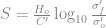
The solution is in the form (similar to that presented in Verruijt) of
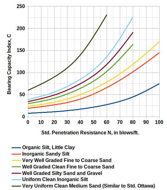
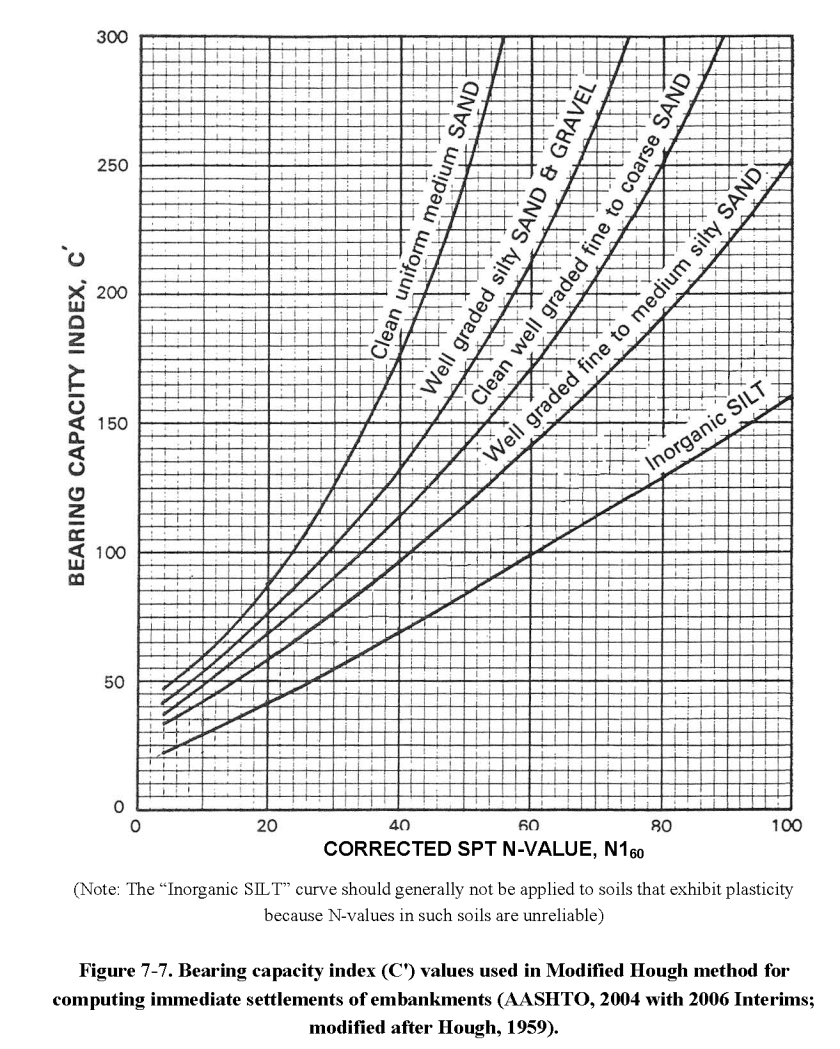
The coefficient is determined using a chart which is below.
The chart itself is basically the same as the one in Hough (1959,) but now things get complicated.
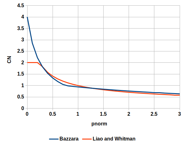
Cheney and Chassie (2000) recommend that the SPT blowcounts be corrected for overburden pressure before correlating the N-values to the bearing capacity index, C′. An overburden correction by Bazaraa (1967) was recommended by Cheney and Chassie (2000). Since that time, many researchers have studied the effect of overburden stress on the SPT N-value, largely in support of liquefaction hazard assessment procedures. Recent consensus by the 1996 and 1998 National Center for Earthquake Engineering Research (NCEER) (Youd et al., 2001) concluded that the correction proposed by Liao & Whitman (1986) (shown in Figure 5-18) could be used for routine engineering applications. Therefore, the correction by Liao & Whitman is included here as part of the Hough procedure, in particular because it is easy to calculate and can be used without charts in simple computation spreadsheets.
The basic problem with this is that Hough himself never mentions any kind of correction for the variations of the SPT tests, overburden or otherwise, and that in modifying Hough’s Method we run the risk of making some assumptions that may not be applicable.
The idea of using the SPT tests, even with shallow foundations in cohesionless soils such as the ones Hough is concerned about, is admirable on the face because undisturbed samples of these soils are hard to obtain in normal soil testing. The problem with SPT tests–which were coming into acceptance when Hough presented his original method–is that their variations in both configuration and those induced by the overburden are significant. It wasn’t until the 1980’s that this was “formally” sorted out with the correction system that we have today.
With our current method we have two stages of correction. The first stage is for variations in the configuration of the split spoon, the effect of the rod and borehole, and most importantly the efficiency of the hammer itself. The second is for the overburden. In both his original paper and the presentation of the method in the Second Edition of his textbook Basic Soils Engineering (1969,) Hough does not delve into either of these.
The whole point of the N60 correction (the first series) was to harmonise the results to a single mechanical standard, and one that was generally attained “back in the day” so that empirical methods such as Hough’s could be used today. We could assume that Hough’s value are at least N60 values, although we’re not guaranteed of that due to the lack of supporting data.
The business of overburden correction brings up Bazaraa (1967.) At this point credit needs to be given where credit is due: Bazaraa had the thankless task of sorting out the settlement methods which were current in his day, and that task included dealing with the variations of the SPT method. Since his overburden correction method was originally used with Hough’s Method and then changed, let us compare the two. We start be defining
The two correction factors for overburden are shown below.
Except for the region where Liao and Whitman is “flat topped” the two are reasonably close, and so substituting Liao and Whitman’s correction is legitimate, assuming it should be used at all.
It should be noted, however, that Bazaraa’s objective is not to correct Hough’s method, which he did not do: it was to provide a new method of estimating settlements in cohesionless soils, and to advance Terzaghi and Peck’s 1948 method. So we are still “up in the air” about how to apply all of this to Hough’s Method.
If the overburden stress is less than the standard atmospheric pressure (approx. 2 ksf) then the N value used will be increased, the C’ values will likewise increase, and the estimated settlement will decrease, which may be more accurate but moves away from conservatism. If the opposite is true then the result will be more conservative. For shallow foundations such as Hough’s Method the lower overburden stresses will be more of a factor (depending upon the depth D.) At this point it is not clear to me (at least) that including an overburden correction is really significant given the other unsolved problems that exist with this method.
One further complicating factor is that, in the aforementioned Second Edition of Basic Soils Engineering, Hough presents a new chart (again with no explanation of correction of any kind) which is redrawn as follows:
Very Uniform Clean Medium Sand (Similar to Std. Ottawa)
58.66
0.0225
It should be noted that, where the curves are directly comparable with Hough (1959), they tend to be lower, i.e., the values of C are less. This would increase settlement and thus conservatism. At this point perhaps we should consider Hough’s Methods in the plural rather than the singular.
We have the conventional Cc based on either liquid limit, initial void ratio or water content. Hough is represented here as well; however, these correlations are for cohesive soils. Hough himself had a broader application for these.
In the Second Edition of Basic Soils Engineering, he presents a function to compute Cc as follows:
He also establishes a relationship between correlations based on liquid limit and those on void ratio, but getting to that is for another time.
In any case he presents values for this equation which are tabulated below, and include both cohesionless and cohesive soils.
a
b*
Uniform cohesionless Material (Cu < 2)
Clean Gravel
0.05
0.5
Coarse Sand
0.06
Medium Sand
0.07
Fine Sand
0.08
Inorganic Silt
0.1
Well-graded, cohesionless soil
Silty sand and gravel
0.09
0.2
Clean, coarse to fine sand
0.12
0.35
Coarse to fine silty sand
0.15
0.25
Sandy silt (inorganic)
0.18
0.25
Inorganic, cohesive soil
Silt, some clay; silty clay; clay
0.29
0.27
Organic, fine-grained soil
Organic silt, little clay
0.35
0.5
*The value of the constant b should be taken as emin whenever the latter is known or can conveniently be determined. Otherwise, use tabulated values as a rough estimate.
From here we can use the well-tried “Cc” formulae (which would include preconsolidated soils) to estimate settlement. This opens up a new vista for using conventional consolidation settlement theory to estimate the settlements of cohesionless soils.
To return to our original objectives, settlement and bearing capacity are, in the process of failure, two sides of the same thing. It is also worth noting that most foundations fail in settlement, although the failure isn’t as “spectacular” as bearing capacity.
The only way to treat them together is to use a method that can combines both phenomena, and finite element methods are capable of doing that. However our profession has been uncomfortable with “black box” methods such as these, although they really apply the same laws we use to formulate closed form solutions. In that respect they have value, and to apply methods such as Hough’s to cohesionless soils with better calibration of the constants would be a good step forward.
References
Bazaraa, A.R.S. (1967). “Use of the Standard Penetration Test for Estimating Settlements of Shallow Foundations on Sand,” Ph.D. Thesis presented to University of Illinois, Urbana.
Hough, B.K. (1959). “Compressibilty as the Basis for Soil Bearing Value,” Journal of the Soil Mechanics and Foundations Division, ASCE, Vol. 85, Part 2.
Hough, B.K. (1969). Basic Soils Engineering. Second Edition. New York: Ronald Press Company.
Professor Bengt Baltzar Broms, Stockholm, Sweden, passed away at the age of 95. He is survived by his wife Carina and children Erik, Karin, and Peter.
Bengt Broms was a leading figure in Swedish and International Geotechnology and Foundation Engineering. He is mourned by many colleagues around the world, especially his former doctoral students, whom he mentored with exceptional expertise and generous advice.
N .A. Tsytovich and Ya.A. Kronik U.S. Army Corps of Engineers, Cold Regions Research and Engineering Laboratory Draft Translation TL-602 February 1977
This article will review some of the initial results of complex cryopedological research based on the physio-chemistry, physics, and mechanics of frozen soils, conducted by the Mechanics of Soils, Bases, and Foundations Section of the Department of Hydraulic Engineering at the V.V. Kuybyshev Moscow Construction Engineering Institute.
This manual provides criteria and guidance for design of foundations for structures for military facilities in arctic and subarctic regions.
The design, construction and maintenance of foundations in these environments are all affected by special environmental conditions. These conditions typically include the following, as applicable:
Seasonal freezing and thawing of ground with attendant frost heaving and other effects.
Occurrence of permanently frozen ground subject to thawing and subsidence during and following construction.
Special physical behavior and properties of frozen soil, rock, and construction materials at low temperatures and under freeze-thaw action.
Difficulty of excavating and handling frozen ground. Poor drainage and possible excess of water during thaw caused by the presence of impervious frozen ground at shallow depths.
Thermal stresses and cracking. Ice uplift and thrust action. Limited availability of natural construction materials, support facilities, and labor.
Adverse conditions of temperature, wind, precipitation, distance, accessibility, working seasons, and cost.
While these factors are important in many other types of construction such as pavements and utilities, they merit separate consideration for foundations for structures.
N.V. Ukhova U.S. Army Corps of Engineers, Cold Regions Research and Engineering Laboratory Draft Translation TL-665 November 1977
The specific characteristics of hydraulic engineering construction on permafrost foundations under harsh climatic conditions result in a situation which the most economic type of dam in the regions is the type made o f local materials. A distinction can be made between two methods of constructing dams from local materials on permafrost foundations : the “warm” method , used when construction takes place primarily during the summertime by usual methods , and usually encountered in regions with moderate climates, and “cold,” when construction takes place in winter with stratified freezing o f the entire dam or its individual elements, or in summer, with subsequent freezing of the structure. The frozen part of the dam is intended to make it impermeable to water. Reliable operation of partly or completely frozen dams is determined by t he temperature regime of the construction and the foundation, which must be such that the frozen “curtain” in the dam does not thaw out during the latter’s operation. The dissertation is devoted to an analytical experimental study of the non-stationary temperature regime of frozen dams made of local materials on permafrost foundations, and constitute one aspect of the problem of construction of dams on permafrost foundations, analyzed by the group of coworkers of the department under the leadership of Corresponding Member of the Academy of Sciences of the USSR, Doctor of Technical Sciences, Professor N.A. Tsytovich. The dissertation consists of four chapters.
N.A. Tsytovich, V.A. Vesilov and N.V. Styrova U.S. Army Corps of Engineers, Cold Regions Research and Engineering Laboratory Draft Translation TL-661 November 1977
This report discusses constructing rock-fill dams with ice cores in the Soviet Union where permafrost soil occurs.
Brian Zelenko, P.E., Erik Loehr, Ph.D., P.E., Andy Boeckmann, P.E., Chris Dorney, AICP, and Elizabeth Godfrey, P.E. WSP USA, Inc. FHWA-HIF-23-008 February 2023
Geohazards—such as landslides, liquefaction, rockfalls, subsidence, expansive/collapsible soils, and erosion—can pose major threats to transportation assets. Extreme weather events can also trigger and/or exacerbate geohazards, and the increasing incidence of such events is a concern in certain regions of the United States. A geohazards management program that evaluates the associated risk can help transportation agencies manage these threats by making comprehensive system performance decisions. Such a program can help agencies manage cost-effective methods for characterizing and reducing risk, develop adaptation methods, and establish a resilient transportation system.
Betsy Godfrey, Brian Zelenko, P.E., Erik Loehr, Ph.D., P.E. Parsons Brinckerhoff FHWA-HIF-23-009 May 2016, updated February 2023
A Peer Exchange was held March 22–23, 2016, in Atlanta, Georgia, to gather experts from different fields relating to geologic hazards, climate change, extreme weather events, and geotechnical asset management (GAM). The purpose was to share perspectives and brainstorm ideas on how FHWA can best continue its geologic hazards program and research. Feedback from the Peer Exchange contributed to updating a draft work plan from Phase I of this study on geohazards, extreme weather events and climate change resilience. The Peer Exchange consisted of presentations from attendees, discussion based on these presentations, breakout sessions for more focused discussion, and brainstorming about suggested changes to the provided draft work plan for a future Phase III study on geologic hazards, extreme events, and climate change. This report provides a summary of the Peer Exchange meeting.




 is determined using a chart which is below.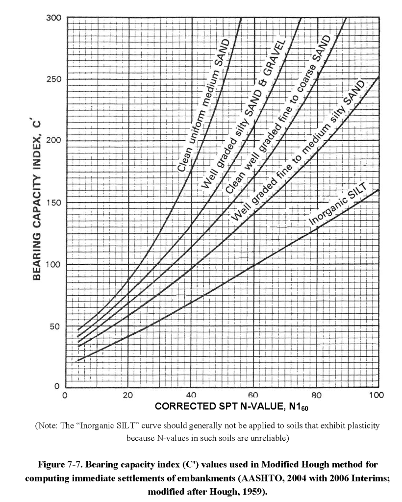

 for overburden are shown below.