Strange Results: The Case of Settlements on Non-Infinite Elastic Half Spaces and Flexible Foundations

In our earlier post Analytical Boussinesq Solutions for Strip, Square and Rectangular Loads we discussed the stress under and settlement of foundations (mostly flexible) on a semi-infinite half space. Usually, though, a hard/competent layer intervenes to mess things up. Some of the books offered on this site–in print and download–have solutions for this problem. Unfortunately unexpected things happen when we consider these things carefully.

To illustrate this, let’s start with the table and diagram below, from NAVFAC DM 7.01.

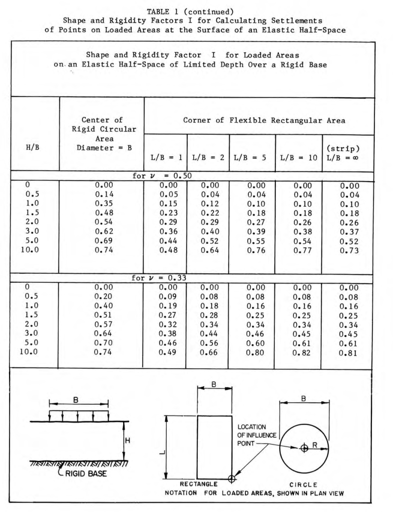
Table 1. Shape and Rigidity Factors I for Calculating Settlements of Points on Loaded Area at the Surface of a Limited Elastic Half-Space (from NAVFAC DM 7.01)

The settlement at the centre of the full foundation (sum of the corners of the divided foundation, see below) is given by the equation

$\delta_v = NqB' \frac {1-\nu_s^2}{E_s} I$ (1)

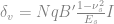
where

$N =$ number of partial foundations used to compute total settlement (with centre settlements, usually $N = 4$
$q =$ uniform load on foundation
$B' =$ small dimension of partial foundation
$\nu_s =$ Poisson’s Ratio of soil
$E_s =$ Young’s Modulus of soil
$I =$ influence coefficient

Note that note that we’re now dealing with settlements. The soil being compressed is limited to a height H from the surface to the “rigid base.” In this diagram we do this corner by corner, as we did for the stresses in Analytical Boussinesq Solutions for Strip, Square and Rectangular Loads. In both this and Going Around in Circles for Rigid and Flexible Foundations we used another chart, which is shown below.

Table 2. Values for the influence coefficients omega (from Tsytovich (1976))

The two charts differ as follows:

Both use Equation (1), albeit differently, as described immediately below.
The basic formula is the same but the influence coefficient notation is different; the DM 7.01 chart uses I while the Tsytovich chart uses $\omega$ .
The settlement is presented differently; the DM 7.01 chart shows it at the centre of the circular foundation and the corner of the rectangles while the Tsytovich charts shows an average settlement. For the Tsytovich chart, the dimension B’ should be replaced by b, the full small dimension of the foundation, and L’ by l, the full large dimension of the foundation. In this case $\alpha = \frac{l}{b}$ .

Let us look at an example, from NAVFAC DM 7.01.

Table 3. Example of Shape and Rigidity Factors I for Calculating Settlements of Points on Loaded Area at the Surface of an Elastic Half-Space (from NAVFAC DM 7.01)

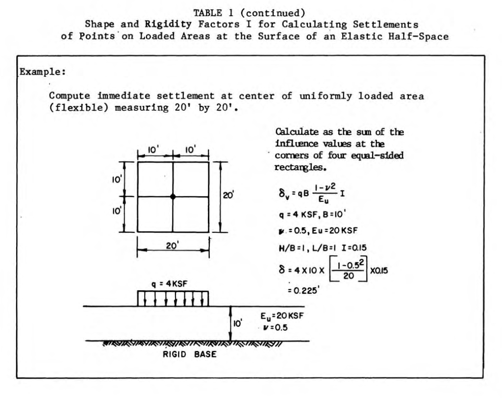
As was the case with the stresses in Analytical Boussinesq Solutions for Strip, Square and Rectangular Loads, we use the corners and divide up the entire foundation into four (4) identical foundations. The influence coefficients shown in the DM 7.01 chart above are used. The maximum deflection (at the centre) is thus four times the partial corner deflections.

Here’s where we run into the first problem: the example is wrong because it only considers the corner deflection of one partial foundation. The problem statement implies that, if we add all four partial foundations touching the corners of the partial foundations (which are all at the centre of the full one) we would get the complete settlement at the centre. Doing this yields 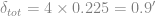$\delta_{tot} = 4 \times 0.225 = 0.9'$ .

If we use the Tsytovich chart we can compute the average deflection of the foundation, and we can use the entire foundation at one time. We first note that $\alpha = \frac{l}{b} = \frac{20}{20} = 1$ . We then note that $\frac{h}{b} = \frac{10}{20} = 0.5$ . From the Tsytovich chart $\omega_{mh} = 0.39$ and the settlement as follows:

$\delta_{mh} = 4 \times 20 \times \frac{1-0.5^2}{20} \times 0.39 = 1.17'$ (2)

Although “average” results can be different based on the method of averaging (something students frequently overlook,) it makes sense that a average result should be somewhat below the deflection at the centre. That’s not the case here.

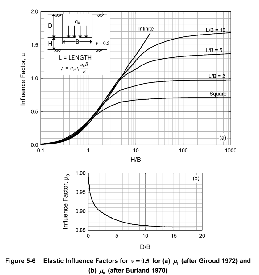
So let’s turn to the newer NAVFAC DM 7.1. They replaced the above chart with the following for settlements:

Figure 1. Elastic Influence Factors for Poisson’s Ratio = 1/2. (a) for mu1, (b) for mu0.

To start with, Figure 5-6 (and the accompanying text) really don’t say whether it’s settlement at the corners, centre or an average settlement. Giroud (1972), the source of Figure 5-6a, does say that it is a corner settlement similar in concept to the old DM 7.01, but the new document does not make this clear. From this, H/B = 10/10 = 1 and L/B = 1. Looking at the chart $\mu_1 = 0.35$ and summing the corner displacements of the partial foundations,

$\rho = 4 \times 1 \times 0.35 \times \frac {4 \times 10}{20} = 2.8'$ (3)

This is significantly different than the old DM 7.01. It is larger than the average settlement shown in the Tsytovich table. But can it be checked against another method?

The answer is “yes,” and to do so we turn to Das (2007). Let us begin by defining the reduced foundation dimensions as B’ and L’, which are obviously half each of B and L. The displacement at the centre of the foundation (the corners of the reduced foundations added together) is thus

$\delta_v = NqB' \frac {1-nu_s^2}{E_s} I_s I_f$ (4)

In this case there are two influence factors, and they correspond with those given in NAVFAC DM 7.1 Figure 5-6: $I_s$ with $\mu_1$ and $I_f$ with $\mu_0$ . We can dispense with the latter by noting that, for the case with no embedment ( $D_f = 0 ,\,I_f = 1$ in a similar way to $\mu_0$ above. (Das gives charts, which we do not reproduce here.) Let us then define

$m = \frac{L'}{B'}$ (5)

and

$n = \frac{H}{B'}$ (6)

Using these ratios, we can define two quantities

$F_1 = \left(m\ln ({\frac {\left (1+\sqrt {{m}^{2}+1}\right )\sqrt {{m}^{2}+{n}^{2}}}{m\left (1+\sqrt {{m}^{2}+{n}^{2}+1}\right )}})+\ln ({\frac {\left (m+\sqrt {{m}^{2}+1}\right )\sqrt {1+{n}^{2}}}{m+\sqrt {{m}^{2}+{n}^{2}+1}}})\right){\pi }^{-1}$ (7)

$F_2 = 1/2\,n\arctan({\frac {m}{n\sqrt {{m}^{2}+{n}^{2}+1}}}){\pi }^{-1}$ (8)

From these quantities,

$I_s = F_1 + \frac{2-\nu}{1-\nu}F_2$ (9)

For our example m = 10/10 = 1 and n = 10/10 = 1. For $\nu = 0.5$ (problem statement,) substituting and solving into Equations (4-8) yields the following:

$F_1 = 0.142$
$F_2 = 0.083$
$I_s = 0.392$

Substituting this yields 2.352′, which is reasonably close to the NAVFAC DM 7.1 solution, and still greater than the solution from Tsytovich.

Notes

The NAVFAC DM 7.1 solution is restricted to values of $\nu = 0.5 $. This is unreasonable; this assumes that the soil is a fluid. It also created a singularity in The Equivalent Thickness Method for Estimating Elastic Settlements.
This shows that even with as venerable a document as NAVFAC DM 7.01 errors can arise, and this should be considered with any book or paper. It also shows that, even with a “cut and dried” topic like theory of elasticity, variations can arise.
All of these solutions are shown in our Elastic Solutions Spreadsheet.
The charts in Das for $I_f = \mu_0$ are similar to the second chart in Figure 1, except that they vary for Poisson’s Ratio and the aspect ratio for the foundation.

References

Das, B.M. (2007) Principles of Foundation Engineering. Sixth Edition. Toronto, Ontario: Thompson.
Giroud, J.-P. 1972. “Settlement of Rectangular Foundation on Soil Layer.” Journal of the Soil Mechanics and Foundations Division, 98(SM1), 149-154.