The Equivalent Thickness Method for Estimating Elastic Settlements

In our very popular post Analytical Boussinesq Solutions for Strip, Square and Rectangular Loads we discuss the use of the theory of elasticity (as originally formulated by Boussinesq) to estimate the stresses and settlements under foundations. We start by giving methods of estimating the stresses under various configurations of rectangular foundations (the circular ones are discussed in the post Going Around in Circles for Rigid and Flexible Foundations.) We then show the use of superposition to expand the use of these results for complex foundations (with further discussion in our post Superposition, and Using Point Loads in Place of Distributed Ones.) We then show the estimation of deflections for simple rigid and flexible foundations. But when it comes to deflections for more complex situations…crickets.

This post is an attempt to solve the “crickets” problem through the use of a method shown in Tsytovich (1976). It’s doubtless useful for preliminary calculations and to enhance our understanding of how settlements of foundations in one place can affect adjacent structures. It also uses some of the linkage between elastic and consolidation settlement theory which is discussed in From Elasticity to Consolidation Settlement: Resolving the Issue of Jean-Louis Briaud’s “Pet Peeve”.

Let us start with Equation (4) of the last linked post, namely

$\epsilon_{{x}}={\frac {p\beta}{E}}$ (1)

where we swap p for $\sigma_x$ as the vertical pressure.

Now let us define an equivalent height h_eq. Keep in mind that we are assuming that the soil’s reaction to vertical pressure is that of a laterally confined specimen; the equivalent height is the height of that equivalent specimen. Multiplying both sides of Equation (1) by this equivalent height,

$h_{{{\it eq}}}\epsilon_{{x}}={\frac {h_{{{\it eq}}}p\beta}{E}}$ (2)

Since by definition

$\epsilon_x = {\frac {s}{h_{{{\it eq}}}}}$ (3)

where s is the settlement, Equation (1) becomes

$s={\frac {h_{{{\it eq}}}p\beta}{E}}$ (4)

Equation (7) of the last linked post tells us that

$E={\frac {\beta}{m_{{v}}}}$ (5)

where

$\beta = 1-2\,{\frac {{\nu}^{2}}{1-\nu}}$ (7)

Combining Equations (4) and (5) yields

$s=h_{{{\it eq}}}pm_{{v}}$ (8)

To compute the equivalent height, we turn to our post Analytical Boussinesq Solutions for Strip, Square and Rectangular Loads, where we modify the equation presented for the deflection of rectangles and squares with Equation (5) above to obtain

$s={\frac {\omega\,pb\left (1-{\nu}^{2}\right )m_{{v}}}{\beta}}$ (9)

The value of $\omega$ is discussed in that post for squares and rectangles and for circles in Going Around in Circles for Rigid and Flexible Foundations. These are very complex (and in the case of circles have no closed form solution.) For convenience the table for these is reproduced below.

If we equate the right hand sides of Equations (8) and (9) and solve for h_eq, we have at last

$h_{eq} = {\frac {\omega\,b\left (1-{\nu}^{2}\right )}{\beta}}$ (10a)

We can also substitute Equation (7) into Equation (10a) and obtain

$h_{eq} = {\frac {\left (-1+\nu\right )^{2}b\omega}{1-2\,\nu}}$ (10b)

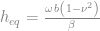
If we define

$A = {\frac {\left (1-\nu\right )^{2}}{1-2\,\nu}}$ (10*)

we can also write the equation thus

$h_{eq} = A\omega b$ (10c)

It should be evident that there are several computational routes to obtain the equivalent height, which is then substituted into Equation (8) to obtain the settlement. Let us consider these options:

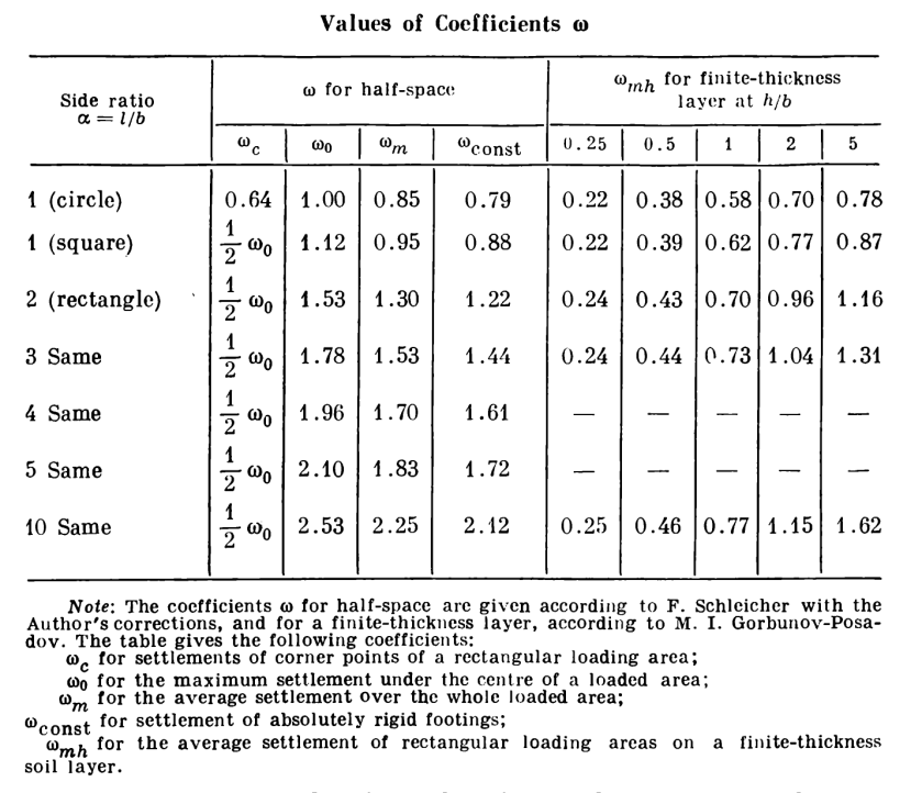
We could tabulate values of $A \omega$ for various foundation configurations and then use these to compute the equivalent height using Equation (10c). This is given in Tsytovich (1976).
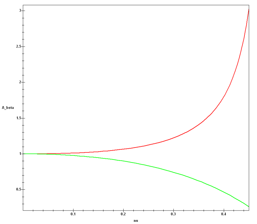
We could determine values for $A$ (it is simply a function of Poisson’s Ratio $\nu$ ), obtain $\omega$ using the table above and then compute the equivalent height using the width of the foundation $b$ . Values for both $A$ and $\beta$ are shown in graphical form as a check for computations.
We could perform direct substitution into Equations (10a) or (10b.) Equation (10a) is probably the best as it will be necessary to compute $\beta$ using Equation (7).

Parameters for Tsytovich Equivalent Thickness Method as a function of Poisson’s Ratio. The red line is the parameter “A” and the green line is the parameter “β”.

Worked Example

As an example, let us consider the same example from the post Analytical Boussinesq Solutions for Strip, Square and Rectangular Loads. The foundation diagram is shown below; we are interested in the settlement at Point A.

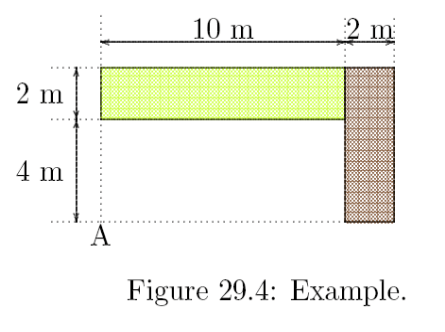
The complete solution is given in the same spreadsheet as the solution for the stress problem, which you can access here. The geometry is the same and the loading is the same: 5 kPa on the yellow (2 m x 10 m foundation) and 15 kPa on the brown foundation (2 m x 6 m.) Keep in mind that, for this method, the value b is always the smaller of the two, and that goes for the “void” foundations as well.

We do not need the depth from the surface; we are only interested in surface deflections. We do need the elastic modulus and Poisson’s Ratio of the soil, which are E = 10,000 kPa and ν = 0.25.

The superposition is exactly the same as before, using the following diagram as before:

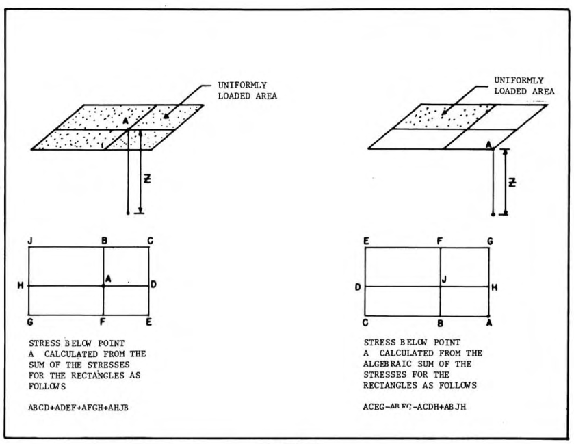
The superposition scheme is as follows:

Yellow Foundation Positive, corners ABFG, pressure +5 kPa
Yellow Foundation Negative, corners ABJH, pressure – 5kPa
Brown Foundation Positive, corners ACEG, pressure +15 kPa
Brown Foundation Negative, corners ABFG, pressure – 15 kPa

We will only go through the calculations for the first one; you can view the spreadsheet for the rest. We proceed as follows:

We compute A and β as follows:
- From Equation (10*), A = (1-0.25)²/(1-(2)(0.25)) = 1.125
- From Equation (7), β = 1-(2)(0.25)²/(1-0.25) = 0.833
- You can verify these using the plot of these parameters.
We compute the coefficient of volume compressibility by using Equation (5), m_v = 0.833/10000 = 0.0000833 1/kPa
We compute the value of α = l/b = 10/6 = 1.6667
We compute the corner value for ω (since we are dealing with corners as was the case with stresses.) We can use the table for ω or we can compute it using the formulae from Analytical Boussinesq Solutions for Strip, Square and Rectangular Loads, but it is ω = 0.71.
We then use Equation (10c) to compute the equivalent height, thus h_eq = (1.125)(0.71)(6) = 4.8 m. This value will be different for each corner point considered.
Using Equation (8), the settlement for this portion of the analysis is s = (4.8)(5)(0.000083333) = 0.002 m = 1.998 mm.

You repeat this process for all four “foundations.” Keep in mind that the negative foundations will result in negative settlements. A summary of the results is as follows:

Yellow Foundation
Rectangle	B, m	L, m	alpha	omega (corner)	heq, m	Pressure p, kPa	Deflection, mm
ABFG (+)	6	10	1.6667	0.71	4.80	5.00	1.998
ABJH (-)	4	10	2.5000	0.83	3.76	-5.00	-1.565
						Total	0.433
Brown Foundation
Rectangle	B, m	L, m	alpha	omega (corner)	heq, m	Pressure p, kPa	Deflection, mm
ACEG (+)	6	12	2.0000	0.77	5.17	15.00	6.462
ABFG (-)	6	10	1.6667	0.71	4.80	-15.00	-5.994
						Total	0.468
						Complete Total	0.901