My institution has featured yet another one of my students who graduated last month, Ogheneruona Uwusiaba, from Nigeria.
“Ruona” (as we called her) was a very diligent student, and took all of the classes I taught (Soil Mechanics, Foundations and Fluid Mechanics Laboratory.) To be a student athlete, mother, engineering student and graduate Magna Cum Laude takes a special type of person, and Ruona is that.
This website–and by extension my teaching–goes around the world to the extent that more visits come from outside the U.S. than inside. Sometimes though the world comes to my classroom, and Ruona was a part of that.
In another post we show the formal, nice way to derive the equations for stresses under point loads. Here we’re going to show a “quick and dirty” way to derive them (or at least some of them.) It’s based on Tsytovich (1976) but I have made some changes to tighten up the theory behind them and make them a little more comprehensible. They don’t derive all of the equations, but the method gives a better physical understanding of what’s going on when we apply such a load to the ground surface.
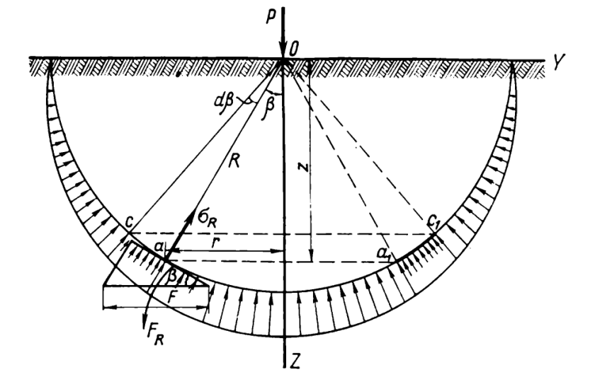
Let’s start with Tsytovich’s diagram, shown below.
Radial stresses under the action of a concentrated force (from Tsytovich (1976))
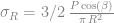
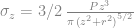
It can be shown that this state exists due to static equilibrium. The point load P forms a sphere around itself; the principal stresses radiate from the load, forming a sphere around the point of radius R. The magnitude of the stress is given by the equation
By same static equilibrium, the vertical force of the stresses and P are thus
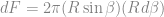
The infinitesimal surface area of the stress can be defined as
Substituting this into the integral yields
Making appropriate substitutions, the integral evaluates to
and thus
Substituting,
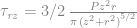
We want the vertical and shear stresses at this point. What we need is a conversion from the polar to cylindrical coordinates, which are given by the equations (Timoshenko and Goodier (1951))
These are coordinate transformations for plane stress equations and are discussed in detail in Boresi et.al. (1993) in terms of the direction cosines of the stress vectors. It may seem odd to see sine terms for these but . If we also assume that , again substituting we have
Since
and
substituting both of these yields our desired result
Many textbooks (such as Verruijt) state these equations in terms of R, but in general problems such as this are defined most simply in terms of the depth of the point of interest z and the horizontal distance from that point r.
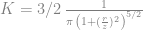
For the vertical stresses, if we define an influence coefficient
then
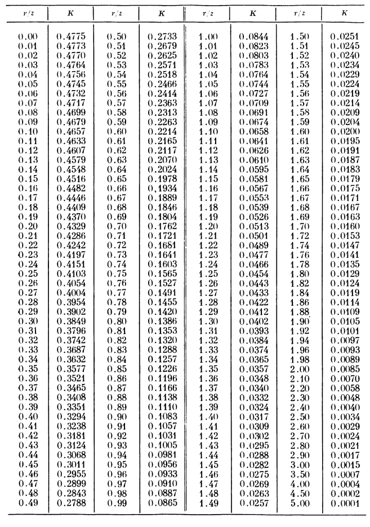
and we can use the following table to determine the influence coefficients K.
Influence Coefficient K to calculate vertical stresses from a concentrated force for a given r/z ratio (from Tsytovich (1976))
The reason we’ve skipped the lateral stresses is because they’re dependent upon the elastic properties of the soil, and also because the vertical stresses are of greater interest.
The point load problem is an important one because many of the area load problems are based on its solution. It can also be used in other ways in spite of the fact that the solution is singular at the point where the load is applied.
Other References
Boresi, A.P., Schmidt, R.J., and Sidebottom, O.M. (1993) Advanced Mechanics of Materials. Fifth Edition. New York: John Wiley and Sons.
Timoshenko, S., and Goodier, J.N. (1951) Theory of Elasticity. New York: McGraww-Hill Book Company, Inc.
Although today we have finite element methods which can combine elastic and plastic components of soil response to loading, the use of lower and upper bound plasticity is important in enhancing our understanding of plasticity in soils and many of the methods we use in geotechnical design. This is an overview of both lower and upper bound solutions to the classic bearing capacity problem. Much of this presentation is drawn from Tsytovich (1976) but the equations have been re-derived and checked.
Lower bound theorem.The true failure load is larger than the load corresponding to an equilibrium system.
Upper bound theorem.The true failure load is smaller than the load corresponding to a mechanism, if that load is determined using the virtual work principle.
For our purposes, since we’re assuming an elastic/perfectly plastic type of soil model, the lower bound solution is where the stress at some point reaches the elastic limit, while the upper bound solution has the stress fully plastic to the boundaries of the system, at which point the capacity of the system to resist further stress has been exhausted (reached its upper limit.)
Assumptions
Foundation is very rigid relative to the soil (for upper bound) and flexible relative to soil (lower bound.) With the latter, a rigid foundation produces infinite stresses at the edges, which means the lower bound solution is zero pressure in that case.
No sliding occurs between foundation and soil (rough foundation)
Applied load is compressive and applied vertically to the centroid of the foundation (upper bound) or uniformly (lower bound)
No applied moments present
Foundation is a strip footing (infinite length)
Soil beneath foundation is homogeneous semi-infinite mass. For the derivations here, we additionally assume that the properties of the soil above the base of the foundation are the same as those below it
Mohr-Coulomb model for soil
General shear failure mode is the governing mode
No soil consolidation occurs
Soil above bottom of foundation has no shear strength; is only a surcharge load against the overturning load
The effective stress of the soil weight acts in a hydrostatic fashion, i.e., the horizontal stresses are the same as the vertical ones.
These are fairly standard assumptions for basic bearing capacity theory; the “additions” from these are workarounds that have been developed. That includes the analysis of finite foundations (squares, rectangles, circles, etc.)
Theory of Elasticity of Infinite Strip Footings
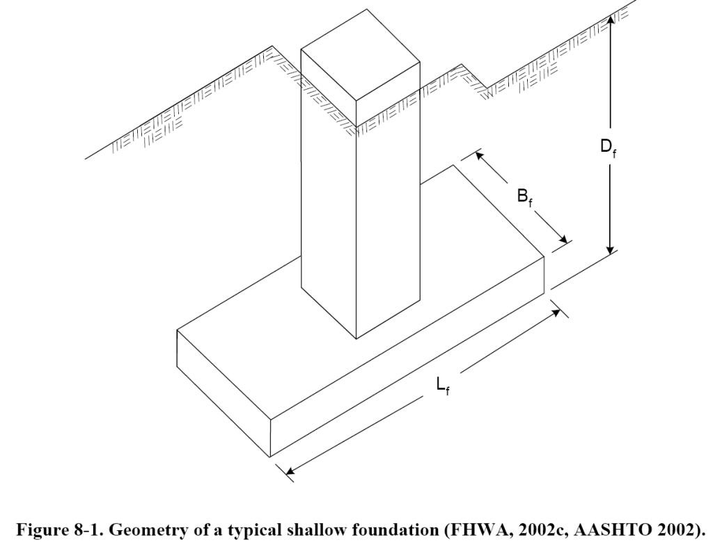
Let us begin by considering the system below of a strip footing with a uniform load. The variables are defined in the figure.
Figure 1 Elastic Model of Stresses of Strip Loads (adapted from Tsytovich (1976))
It can be shown that the stresses at a point of interest can be defined as follows:
(1) (2) (3)
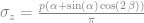
It can also be shown that the principal axis of the stresses at the point are along a line in the middle of the angle . This is the dashed line in the diagram above. Along this line the angle (and thus ) and the principal stresses due to the load become
(4) (5)
Lower Bound Solution
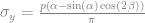
Shallow foundations are seldom built with the base of the foundation at the same elevation as the groundline. They are customarily built to a depth from the surface, as shown below.
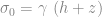
At this point, for analysis purposes, we transform the effect of the depth into an overburden stress, which is the product of the the unit weight of the soil and the depth of the foundation base from the surface D (or h,) as shown below:
Figure 3 Strip Foundation with Surrounding Overburden (from Tsytovich (1976))
The effective stress at any point below the surface is given by the equation
(6)
At the point the hydrostatic stress assumption becomes important. The transformation from Equations (1-3) to (4-5) involved an axis rotation. Assuming the soil acts hydrostatically means that, no matter how we rotate the axis, the addition of the effective stress to the principal stress is independent of direction.
Substituting Equations (7) and (8) into Equation (9) yields
(10)
Solving for z, we have
(11)
At this point we want to find the maximum value of z at which point plasticity first sets in. We do this by taking the derivative of z relative to and setting it to zero, or
(12)
It can be shown that this condition is fulfilled when . Substituting that value back into Equation (11) gives us the value of z at which point plasticity is first induced, or
(13)
If we solve for the pressure , that pressure will be in reality the critical pressure at which plasticity is first induced. Solving for that pressure,
(14)
At this point we need to face reality and note that, if the point we’re looking for is the point at which plastic deformation begins, then it cannot be at any depth other than the base of the foundation, or . Making that final substitution yields at last
(15)
Upper Bound
The upper bound solution is a well-worn path in geotechnical engineering and only the highlights will be shown here.
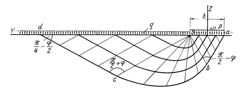
In 1920-1 Prandtl and Reissener solved the problem for a soil by neglecting its own weight, i.e., Equation (6) They determined that the failure pattern and surface can be represented by the following configuration.
Figure 3 Slip Lines and Failure Surface for Upper Bound Bearing Capacity Failure (from Tsytovich (1976))
They determined that the upper bound critical pressure was given by the equation
(16)
If we define
(17)
then
(18)
If we further define
(19)
we have
(20)
The only thing missing from this equation is the effect of the weight of the soil bearing on the failure surface at the bottom of the failure region shown in Figure 3, and thus the bearing capacity equation can be written thus:
(21)
where
(22)
This last bearing capacity factor has been the subject of variable solutions over the years; the one shown here is that of Vesić, which is enshrined in FHWA/AASHTO recommended practice. Verruijt discusses this issue in detail.
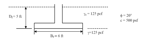
It would probably be useful to state the bearing capacity equations in nomenclature that’s more consistent with American practice (and the diagram above.) In both cases this is, for the lower bound solution,
(15a)
and for the upper bound solution,
(21a)
One important practical difference between the two is the way the overburden is handled. With the lower bound solution, it is equal to , while with the upper bound solution it is simply the pressure . For a uniform soil above the foundation base with no water table to complicate things, .
Direct substitution into Equation (15a) of all of the variables with show that the lower bound critical pressure is 4740.5 psf.
The upper bound is a little more complicated. The three bearing capacity factors are . Substituting these, q and the other variables yield an upper bound critical pressure of 13,436.8 psf.
If the lower bound is a reduction from the upper bound using a factor of safety, then the FS = 2.83. The lower bound solution is conservative.
Conclusion
Although the lower bound solution may be too conservative for general practice, it is at least an interesting exercise to show the variations in critical pressure from the onset of plastic yielding to its final failed state.
First-generation student Arielle Scalioni, a civil engineering major, will be receiving her bachelor’s degree from UTC during upcoming commencement ceremonies.
The survey further asked universities what professional references are being introduced to students during their academic training on ERS. Among the available literature, the most heavily used were FHWA’s Geotechnical Engineering Circulars. Among the most selected circulars were:
All but the first are in our collection (the first isn’t on the FHWA’s site either.) I have taking the liberty of noting that two of those are in print.


 radiate from the load, forming a sphere around the point of radius R. The magnitude of the stress is given by the equation


 . If we also assume that
  , again substituting we have
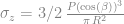


 (1)
(1) (2)
(2) (3)
(3) . This is the dashed line in the diagram above. Along this line the angle
  (and thus
  ) and the principal stresses due to the load become
 (4)
(4) (5)
(5)
 and the depth of the foundation base from the surface D (or h,) as shown below:
 (6)
(6) (7)
(7) (8)
(8) (9)
(9) (10)
(10) (11)
(11) (12)
(12) . Substituting that value back into Equation (11) gives us the value of z at which point plasticity is first induced, or
 (13)
(13) , that pressure will be in reality the critical pressure at which plasticity is first induced. Solving for that pressure,
  (14)
(14) . Making that final substitution yields at last
 (15)
(15)
 (16)
(16) (17)
(17) (18)
(18) (19)
(19) (20)
(20) (21)
(21) (22)
(22)
 (15a)
(15a) (21a)
(21a) , while with the upper bound solution it is simply the pressure
  . For a uniform soil above the foundation base with no water table to complicate things,
  .
. . Substituting these, q and the other variables yield an upper bound critical pressure of 13,436.8 psf.