Our last cases to consider are the cases of uniaxial loading. Although these cases may seem trivial, they are important. As it was with the two-dimensional cases of plane stress and plane strain, there are two variations of the uniaxial loading to consider: uniaxial stress and uniaxial strain.
Uniaxial Stress
We start by considering the constitutive equation of the three-dimensional case, which is
![\left[\begin{array}{cccccc} {\frac{\left(1-\nu\right)\lambda}{\nu}} & \lambda & \lambda & 0 & 0 & 0\\ \noalign{\medskip}\lambda & {\frac{\left(1-\nu\right)\lambda}{\nu}} & \lambda & 0 & 0 & 0\\ \noalign{\medskip}\lambda & \lambda & {\frac{\left(1-\nu\right)\lambda}{\nu}} & 0 & 0 & 0\\ \noalign{\medskip}0 & 0 & 0 & G & 0 & 0\\ \noalign{\medskip}0 & 0 & 0 & 0 & G & 0\\ \noalign{\medskip}0 & 0 & 0 & 0 & 0 & G \end{array}\right]\left[\begin{array}{c} \epsilon_{{x}}\\ \noalign{\medskip}\epsilon_{{y}}\\ \noalign{\medskip}\epsilon_{{z}}\\ \noalign{\medskip}\gamma{}_{{\it xy}}\\ \noalign{\medskip}{\it \gamma}_{{\it yz}}\\ \noalign{\medskip}{\it \gamma}_{{\it zx}} \end{array}\right]=\left[\begin{array}{c} \sigma_{{x}}\\ \noalign{\medskip}\sigma_{{y}}\\ \noalign{\medskip}\sigma_{{z}}\\ \noalign{\medskip}\tau_{{\it xy}}\\ \noalign{\medskip}\tau_{{\it yz}}\\ \noalign{\medskip}\tau_{{\it zx}} \end{array}\right]](https://s0.wp.com/latex.php?latex=%5Cleft%5B%5Cbegin%7Barray%7D%7Bcccccc%7D+%7B%5Cfrac%7B%5Cleft%281-%5Cnu%5Cright%29%5Clambda%7D%7B%5Cnu%7D%7D+%26+%5Clambda+%26+%5Clambda+%26+0+%26+0+%26+0%5C%5C+%5Cnoalign%7B%5Cmedskip%7D%5Clambda+%26+%7B%5Cfrac%7B%5Cleft%281-%5Cnu%5Cright%29%5Clambda%7D%7B%5Cnu%7D%7D+%26+%5Clambda+%26+0+%26+0+%26+0%5C%5C+%5Cnoalign%7B%5Cmedskip%7D%5Clambda+%26+%5Clambda+%26+%7B%5Cfrac%7B%5Cleft%281-%5Cnu%5Cright%29%5Clambda%7D%7B%5Cnu%7D%7D+%26+0+%26+0+%26+0%5C%5C+%5Cnoalign%7B%5Cmedskip%7D0+%26+0+%26+0+%26+G+%26+0+%26+0%5C%5C+%5Cnoalign%7B%5Cmedskip%7D0+%26+0+%26+0+%26+0+%26+G+%26+0%5C%5C+%5Cnoalign%7B%5Cmedskip%7D0+%26+0+%26+0+%26+0+%26+0+%26+G+%5Cend%7Barray%7D%5Cright%5D%5Cleft%5B%5Cbegin%7Barray%7D%7Bc%7D+%5Cepsilon_%7B%7Bx%7D%7D%5C%5C+%5Cnoalign%7B%5Cmedskip%7D%5Cepsilon_%7B%7By%7D%7D%5C%5C+%5Cnoalign%7B%5Cmedskip%7D%5Cepsilon_%7B%7Bz%7D%7D%5C%5C+%5Cnoalign%7B%5Cmedskip%7D%5Cgamma%7B%7D_%7B%7B%5Cit+xy%7D%7D%5C%5C+%5Cnoalign%7B%5Cmedskip%7D%7B%5Cit+%5Cgamma%7D_%7B%7B%5Cit+yz%7D%7D%5C%5C+%5Cnoalign%7B%5Cmedskip%7D%7B%5Cit+%5Cgamma%7D_%7B%7B%5Cit+zx%7D%7D+%5Cend%7Barray%7D%5Cright%5D%3D%5Cleft%5B%5Cbegin%7Barray%7D%7Bc%7D+%5Csigma_%7B%7Bx%7D%7D%5C%5C+%5Cnoalign%7B%5Cmedskip%7D%5Csigma_%7B%7By%7D%7D%5C%5C+%5Cnoalign%7B%5Cmedskip%7D%5Csigma_%7B%7Bz%7D%7D%5C%5C+%5Cnoalign%7B%5Cmedskip%7D%5Ctau_%7B%7B%5Cit+xy%7D%7D%5C%5C+%5Cnoalign%7B%5Cmedskip%7D%5Ctau_%7B%7B%5Cit+yz%7D%7D%5C%5C+%5Cnoalign%7B%5Cmedskip%7D%5Ctau_%7B%7B%5Cit+zx%7D%7D+%5Cend%7Barray%7D%5Cright%5D+&bg=ffffff&fg=777777&s=0&c=20201002)
For uniaxial stress, the following parameters are zero:


As a result, stress and strain vectors are
![\epsilon=\left[\begin{array}{c} \epsilon_{{x}}\\ \noalign{\medskip}\epsilon_{{y}}\\ \noalign{\medskip}\epsilon_{{z}}\\ \noalign{\medskip}0\\ \noalign{\medskip}0\\ \noalign{\medskip}0 \end{array}\right]](https://s0.wp.com/latex.php?latex=%5Cepsilon%3D%5Cleft%5B%5Cbegin%7Barray%7D%7Bc%7D+%5Cepsilon_%7B%7Bx%7D%7D%5C%5C+%5Cnoalign%7B%5Cmedskip%7D%5Cepsilon_%7B%7By%7D%7D%5C%5C+%5Cnoalign%7B%5Cmedskip%7D%5Cepsilon_%7B%7Bz%7D%7D%5C%5C+%5Cnoalign%7B%5Cmedskip%7D0%5C%5C+%5Cnoalign%7B%5Cmedskip%7D0%5C%5C+%5Cnoalign%7B%5Cmedskip%7D0+%5Cend%7Barray%7D%5Cright%5D+&bg=ffffff&fg=777777&s=0&c=20201002)
![\sigma=\left[\begin{array}{c} \sigma_{{x}}\\ \noalign{\medskip}0\\ \noalign{\medskip}0\\ \noalign{\medskip}0\\ \noalign{\medskip}0\\ \noalign{\medskip}0 \end{array}\right]](https://s0.wp.com/latex.php?latex=%5Csigma%3D%5Cleft%5B%5Cbegin%7Barray%7D%7Bc%7D+%5Csigma_%7B%7Bx%7D%7D%5C%5C+%5Cnoalign%7B%5Cmedskip%7D0%5C%5C+%5Cnoalign%7B%5Cmedskip%7D0%5C%5C+%5Cnoalign%7B%5Cmedskip%7D0%5C%5C+%5Cnoalign%7B%5Cmedskip%7D0%5C%5C+%5Cnoalign%7B%5Cmedskip%7D0+%5Cend%7Barray%7D%5Cright%5D+&bg=ffffff&fg=777777&s=0&c=20201002)
It’s worth noting that we’ve zeroed out the shear stresses and strains. That’s because, with a uniaxial loading, the x, y and z stresses and strains are guaranteed to be principal stresses and strains, and thus the shear stresses are zero. We will see that the shear stresses and strains will return with axis rotation.
In any case, doing the usual multiplications and inverse multiplications, we have the following:
![\epsilon=\left[\begin{array}{c} \epsilon_{{x}}\\ \noalign{\medskip}\epsilon_{{y}}\\ \noalign{\medskip}\epsilon_{{z}}\\ \noalign{\medskip}0\\ \noalign{\medskip}0\\ \noalign{\medskip}0 \end{array}\right]=\left[\begin{array}{c} -{\frac{\nu\,\sigma_{{x}}}{\lambda\,\left(-1+\nu+2\,{\nu}^{2}\right)}}\\ \noalign{\medskip}{\frac{{\nu}^{2}\sigma_{{x}}}{\lambda\,\left(-1+\nu+2\,{\nu}^{2}\right)}}\\ \noalign{\medskip}{\frac{{\nu}^{2}\sigma_{{x}}}{\lambda\,\left(-1+\nu+2\,{\nu}^{2}\right)}}\\ \noalign{\medskip}0\\ \noalign{\medskip}0\\ \noalign{\medskip}0 \end{array}\right]](https://s0.wp.com/latex.php?latex=%5Cepsilon%3D%5Cleft%5B%5Cbegin%7Barray%7D%7Bc%7D+%5Cepsilon_%7B%7Bx%7D%7D%5C%5C+%5Cnoalign%7B%5Cmedskip%7D%5Cepsilon_%7B%7By%7D%7D%5C%5C+%5Cnoalign%7B%5Cmedskip%7D%5Cepsilon_%7B%7Bz%7D%7D%5C%5C+%5Cnoalign%7B%5Cmedskip%7D0%5C%5C+%5Cnoalign%7B%5Cmedskip%7D0%5C%5C+%5Cnoalign%7B%5Cmedskip%7D0+%5Cend%7Barray%7D%5Cright%5D%3D%5Cleft%5B%5Cbegin%7Barray%7D%7Bc%7D+-%7B%5Cfrac%7B%5Cnu%5C%2C%5Csigma_%7B%7Bx%7D%7D%7D%7B%5Clambda%5C%2C%5Cleft%28-1%2B%5Cnu%2B2%5C%2C%7B%5Cnu%7D%5E%7B2%7D%5Cright%29%7D%7D%5C%5C+%5Cnoalign%7B%5Cmedskip%7D%7B%5Cfrac%7B%7B%5Cnu%7D%5E%7B2%7D%5Csigma_%7B%7Bx%7D%7D%7D%7B%5Clambda%5C%2C%5Cleft%28-1%2B%5Cnu%2B2%5C%2C%7B%5Cnu%7D%5E%7B2%7D%5Cright%29%7D%7D%5C%5C+%5Cnoalign%7B%5Cmedskip%7D%7B%5Cfrac%7B%7B%5Cnu%7D%5E%7B2%7D%5Csigma_%7B%7Bx%7D%7D%7D%7B%5Clambda%5C%2C%5Cleft%28-1%2B%5Cnu%2B2%5C%2C%7B%5Cnu%7D%5E%7B2%7D%5Cright%29%7D%7D%5C%5C+%5Cnoalign%7B%5Cmedskip%7D0%5C%5C+%5Cnoalign%7B%5Cmedskip%7D0%5C%5C+%5Cnoalign%7B%5Cmedskip%7D0+%5Cend%7Barray%7D%5Cright%5D+&bg=ffffff&fg=777777&s=0&c=20201002)
![\sigma=\left[\begin{array}{c} \sigma_{{x}}\\ \noalign{\medskip}0\\ \noalign{\medskip}0\\ \noalign{\medskip}0\\ \noalign{\medskip}0\\ \noalign{\medskip}0 \end{array}\right]=\left[\begin{array}{c} {\frac{\left(1-\nu\right)\lambda\,\epsilon_{{x}}}{\nu}}+\lambda\,\epsilon_{{y}}+\lambda\,\epsilon_{{z}}\\ \noalign{\medskip}\lambda\,\epsilon_{{x}}+{\frac{\left(1-\nu\right)\lambda\,\epsilon_{{y}}}{\nu}}+\lambda\,\epsilon_{{z}}\\ \noalign{\medskip}\lambda\,\epsilon_{{x}}+\lambda\,\epsilon_{{y}}+{\frac{\left(1-\nu\right)\lambda\,\epsilon_{{z}}}{\nu}}\\ \noalign{\medskip}0\\ \noalign{\medskip}0\\ \noalign{\medskip}0 \end{array}\right]](https://s0.wp.com/latex.php?latex=%5Csigma%3D%5Cleft%5B%5Cbegin%7Barray%7D%7Bc%7D+%5Csigma_%7B%7Bx%7D%7D%5C%5C+%5Cnoalign%7B%5Cmedskip%7D0%5C%5C+%5Cnoalign%7B%5Cmedskip%7D0%5C%5C+%5Cnoalign%7B%5Cmedskip%7D0%5C%5C+%5Cnoalign%7B%5Cmedskip%7D0%5C%5C+%5Cnoalign%7B%5Cmedskip%7D0+%5Cend%7Barray%7D%5Cright%5D%3D%5Cleft%5B%5Cbegin%7Barray%7D%7Bc%7D+%7B%5Cfrac%7B%5Cleft%281-%5Cnu%5Cright%29%5Clambda%5C%2C%5Cepsilon_%7B%7Bx%7D%7D%7D%7B%5Cnu%7D%7D%2B%5Clambda%5C%2C%5Cepsilon_%7B%7By%7D%7D%2B%5Clambda%5C%2C%5Cepsilon_%7B%7Bz%7D%7D%5C%5C+%5Cnoalign%7B%5Cmedskip%7D%5Clambda%5C%2C%5Cepsilon_%7B%7Bx%7D%7D%2B%7B%5Cfrac%7B%5Cleft%281-%5Cnu%5Cright%29%5Clambda%5C%2C%5Cepsilon_%7B%7By%7D%7D%7D%7B%5Cnu%7D%7D%2B%5Clambda%5C%2C%5Cepsilon_%7B%7Bz%7D%7D%5C%5C+%5Cnoalign%7B%5Cmedskip%7D%5Clambda%5C%2C%5Cepsilon_%7B%7Bx%7D%7D%2B%5Clambda%5C%2C%5Cepsilon_%7B%7By%7D%7D%2B%7B%5Cfrac%7B%5Cleft%281-%5Cnu%5Cright%29%5Clambda%5C%2C%5Cepsilon_%7B%7Bz%7D%7D%7D%7B%5Cnu%7D%7D%5C%5C+%5Cnoalign%7B%5Cmedskip%7D0%5C%5C+%5Cnoalign%7B%5Cmedskip%7D0%5C%5C+%5Cnoalign%7B%5Cmedskip%7D0+%5Cend%7Barray%7D%5Cright%5D+&bg=ffffff&fg=777777&s=0&c=20201002)
Considering the first rows of Equation (5) gives us

and from the next two rows

It’s possible to formulate the computation of the stresses based on the strains, but in uniaxial loading it is usually easier to know the stresses first.
Although uniaxial loading is common in tensile and compressive stresses of materials such as metals and plastics, in geotechnical engineering it is mainly concentrated in two types of tests: Triaxial tests and Unconfined Compression (UC) tests. Since in Mohr-Coulomb theory we use a maximum shear stress to determine the point of failure, and the shear stresses and strains don’t appear in the above equations, an explanation as to how shear stresses and strains apply is reasonable.
Rather than go into a math-intensive derivation of the problem, recourse to Mohr’s Circle is more instructive.
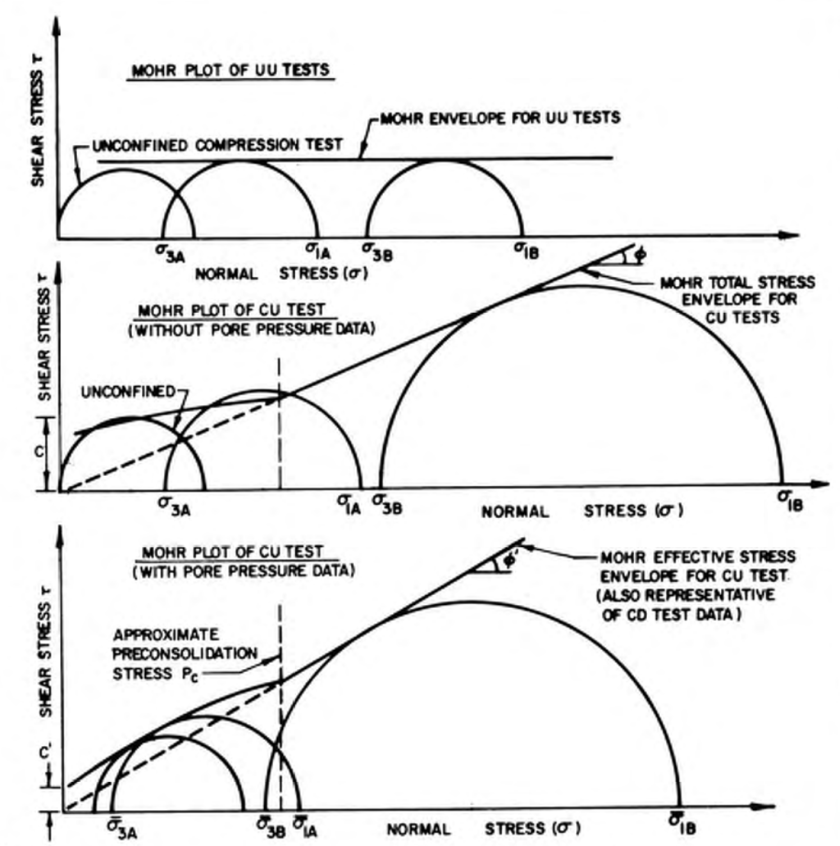
Let’s look at the top diagram from a UC test. The main uniaxial stress 

In the case of materials with internal friction, things are a little more complicated, because the angle from the principal stress to the point where Mohr’s Circle meets the failure envelope is greater than 90 degrees, thus the angle between the centre axis and the failure plane is greater than 45 degrees, and depends upon the interaction of the cohesion and the internal friction angle.
Of course people who actually run these tests will tell you that these specimens don’t always fail along these planes, or simply bulge at failure. That’s because soils don’t always obey Mohr-Coulomb elastic-perfectly plastic failure theory, which is one of those things that makes geotechnical engineering challenging.
Uniaxial Strain
Although this case doesn’t seem at first glance to be very useful, it’s really an important one for geotechnical engineers. We’ll start again with Equation (1) and zero out the following parameters:

Of course Equation (2b) applies as well. Doing this results in the following vectors, and I’ll go ahead and multiply and inversely multiply through as before:
![\epsilon=\left[\begin{array}{c} \epsilon_{{x}}\\ \noalign{\medskip}0\\ \noalign{\medskip}0\\ \noalign{\medskip}0\\ \noalign{\medskip}0\\ \noalign{\medskip}0 \end{array}\right]=\left[\begin{array}{c} -{\frac{\nu\,\sigma_{{x}}}{\lambda\,\left(-1+\nu+2\,{\nu}^{2}\right)}}+{\frac{{\nu}^{2}\sigma_{{y}}}{\lambda\,\left(-1+\nu+2\,{\nu}^{2}\right)}}+{\frac{{\nu}^{2}\sigma_{{z}}}{\lambda\,\left(-1+\nu+2\,{\nu}^{2}\right)}}\\ \noalign{\medskip}{\frac{{\nu}^{2}\sigma_{{x}}}{\lambda\,\left(-1+\nu+2\,{\nu}^{2}\right)}}-{\frac{\nu\,\sigma_{{y}}}{\lambda\,\left(-1+\nu+2\,{\nu}^{2}\right)}}+{\frac{{\nu}^{2}\sigma_{{z}}}{\lambda\,\left(-1+\nu+2\,{\nu}^{2}\right)}}\\ \noalign{\medskip}{\frac{{\nu}^{2}\sigma_{{x}}}{\lambda\,\left(-1+\nu+2\,{\nu}^{2}\right)}}+{\frac{{\nu}^{2}\sigma_{{y}}}{\lambda\,\left(-1+\nu+2\,{\nu}^{2}\right)}}-{\frac{\nu\,\sigma_{{z}}}{\lambda\,\left(-1+\nu+2\,{\nu}^{2}\right)}}\\ \noalign{\medskip}0\\ \noalign{\medskip}0\\ \noalign{\medskip}0 \end{array}\right]](https://s0.wp.com/latex.php?latex=%5Cepsilon%3D%5Cleft%5B%5Cbegin%7Barray%7D%7Bc%7D+%5Cepsilon_%7B%7Bx%7D%7D%5C%5C+%5Cnoalign%7B%5Cmedskip%7D0%5C%5C+%5Cnoalign%7B%5Cmedskip%7D0%5C%5C+%5Cnoalign%7B%5Cmedskip%7D0%5C%5C+%5Cnoalign%7B%5Cmedskip%7D0%5C%5C+%5Cnoalign%7B%5Cmedskip%7D0+%5Cend%7Barray%7D%5Cright%5D%3D%5Cleft%5B%5Cbegin%7Barray%7D%7Bc%7D+-%7B%5Cfrac%7B%5Cnu%5C%2C%5Csigma_%7B%7Bx%7D%7D%7D%7B%5Clambda%5C%2C%5Cleft%28-1%2B%5Cnu%2B2%5C%2C%7B%5Cnu%7D%5E%7B2%7D%5Cright%29%7D%7D%2B%7B%5Cfrac%7B%7B%5Cnu%7D%5E%7B2%7D%5Csigma_%7B%7By%7D%7D%7D%7B%5Clambda%5C%2C%5Cleft%28-1%2B%5Cnu%2B2%5C%2C%7B%5Cnu%7D%5E%7B2%7D%5Cright%29%7D%7D%2B%7B%5Cfrac%7B%7B%5Cnu%7D%5E%7B2%7D%5Csigma_%7B%7Bz%7D%7D%7D%7B%5Clambda%5C%2C%5Cleft%28-1%2B%5Cnu%2B2%5C%2C%7B%5Cnu%7D%5E%7B2%7D%5Cright%29%7D%7D%5C%5C+%5Cnoalign%7B%5Cmedskip%7D%7B%5Cfrac%7B%7B%5Cnu%7D%5E%7B2%7D%5Csigma_%7B%7Bx%7D%7D%7D%7B%5Clambda%5C%2C%5Cleft%28-1%2B%5Cnu%2B2%5C%2C%7B%5Cnu%7D%5E%7B2%7D%5Cright%29%7D%7D-%7B%5Cfrac%7B%5Cnu%5C%2C%5Csigma_%7B%7By%7D%7D%7D%7B%5Clambda%5C%2C%5Cleft%28-1%2B%5Cnu%2B2%5C%2C%7B%5Cnu%7D%5E%7B2%7D%5Cright%29%7D%7D%2B%7B%5Cfrac%7B%7B%5Cnu%7D%5E%7B2%7D%5Csigma_%7B%7Bz%7D%7D%7D%7B%5Clambda%5C%2C%5Cleft%28-1%2B%5Cnu%2B2%5C%2C%7B%5Cnu%7D%5E%7B2%7D%5Cright%29%7D%7D%5C%5C+%5Cnoalign%7B%5Cmedskip%7D%7B%5Cfrac%7B%7B%5Cnu%7D%5E%7B2%7D%5Csigma_%7B%7Bx%7D%7D%7D%7B%5Clambda%5C%2C%5Cleft%28-1%2B%5Cnu%2B2%5C%2C%7B%5Cnu%7D%5E%7B2%7D%5Cright%29%7D%7D%2B%7B%5Cfrac%7B%7B%5Cnu%7D%5E%7B2%7D%5Csigma_%7B%7By%7D%7D%7D%7B%5Clambda%5C%2C%5Cleft%28-1%2B%5Cnu%2B2%5C%2C%7B%5Cnu%7D%5E%7B2%7D%5Cright%29%7D%7D-%7B%5Cfrac%7B%5Cnu%5C%2C%5Csigma_%7B%7Bz%7D%7D%7D%7B%5Clambda%5C%2C%5Cleft%28-1%2B%5Cnu%2B2%5C%2C%7B%5Cnu%7D%5E%7B2%7D%5Cright%29%7D%7D%5C%5C+%5Cnoalign%7B%5Cmedskip%7D0%5C%5C+%5Cnoalign%7B%5Cmedskip%7D0%5C%5C+%5Cnoalign%7B%5Cmedskip%7D0+%5Cend%7Barray%7D%5Cright%5D+&bg=ffffff&fg=777777&s=0&c=20201002)
![\sigma=\left[\begin{array}{c} \sigma_{{x}}\\ \noalign{\medskip}\sigma_{y}\\ \noalign{\medskip}\sigma_{z}\\ \noalign{\medskip}0\\ \noalign{\medskip}0\\ \noalign{\medskip}0 \end{array}\right]=\left[\begin{array}{c} {\frac{\left(1-\nu\right)\lambda\,\epsilon_{{x}}}{\nu}}\\ \noalign{\medskip}\lambda\,\epsilon_{{x}}\\ \noalign{\medskip}\lambda\,\epsilon_{{x}}\\ \noalign{\medskip}0\\ \noalign{\medskip}0\\ \noalign{\medskip}0 \end{array}\right]](https://s0.wp.com/latex.php?latex=%5Csigma%3D%5Cleft%5B%5Cbegin%7Barray%7D%7Bc%7D+%5Csigma_%7B%7Bx%7D%7D%5C%5C+%5Cnoalign%7B%5Cmedskip%7D%5Csigma_%7By%7D%5C%5C+%5Cnoalign%7B%5Cmedskip%7D%5Csigma_%7Bz%7D%5C%5C+%5Cnoalign%7B%5Cmedskip%7D0%5C%5C+%5Cnoalign%7B%5Cmedskip%7D0%5C%5C+%5Cnoalign%7B%5Cmedskip%7D0+%5Cend%7Barray%7D%5Cright%5D%3D%5Cleft%5B%5Cbegin%7Barray%7D%7Bc%7D+%7B%5Cfrac%7B%5Cleft%281-%5Cnu%5Cright%29%5Clambda%5C%2C%5Cepsilon_%7B%7Bx%7D%7D%7D%7B%5Cnu%7D%7D%5C%5C+%5Cnoalign%7B%5Cmedskip%7D%5Clambda%5C%2C%5Cepsilon_%7B%7Bx%7D%7D%5C%5C+%5Cnoalign%7B%5Cmedskip%7D%5Clambda%5C%2C%5Cepsilon_%7B%7Bx%7D%7D%5C%5C+%5Cnoalign%7B%5Cmedskip%7D0%5C%5C+%5Cnoalign%7B%5Cmedskip%7D0%5C%5C+%5Cnoalign%7B%5Cmedskip%7D0+%5Cend%7Barray%7D%5Cright%5D+&bg=ffffff&fg=777777&s=0&c=20201002)
Extracting the important results,


Although it may seem esoteric, this condition is actually important because it simulates confined specimens under uniaxial load. The best known of these, of course, is consolidation testing and all of the variations of that which are employed. It may seem strange to employ elastic theory in this situation, but that speaks to Jean-Louis Briaud’s pet peeve regarding consolidation testing and the partial solution to the problem he poses. Some discussion of this relationship can also be found in Verruijt.
The whole concept of confined specimens is based on the fact that the entire ground upon which we build is a confined specimen, confined by the semi-infinite soil surrounding the loaded portion. Thus this unlikely looking case is very relevant for real geotechnical engineering.

 (1a)
(1a) (1b)
(1b) (1c)
(1c)![D_{e}=\left[\begin{array}{cccc} {\frac{\left(1-\nu\right)\lambda}{\nu}} & \lambda & \lambda & 0\\ \noalign{\medskip}\lambda & {\frac{\left(1-\nu\right)\lambda}{\nu}} & \lambda & 0\\ \noalign{\medskip}\lambda & \lambda & {\frac{\left(1-\nu\right)\lambda}{\nu}} & 0\\ \noalign{\medskip}0 & 0 & 0 & G \end{array}\right]](https://s0.wp.com/latex.php?latex=D_%7Be%7D%3D%5Cleft%5B%5Cbegin%7Barray%7D%7Bcccc%7D+%7B%5Cfrac%7B%5Cleft%281-%5Cnu%5Cright%29%5Clambda%7D%7B%5Cnu%7D%7D+%26+%5Clambda+%26+%5Clambda+%26+0%5C%5C+%5Cnoalign%7B%5Cmedskip%7D%5Clambda+%26+%7B%5Cfrac%7B%5Cleft%281-%5Cnu%5Cright%29%5Clambda%7D%7B%5Cnu%7D%7D+%26+%5Clambda+%26+0%5C%5C+%5Cnoalign%7B%5Cmedskip%7D%5Clambda+%26+%5Clambda+%26+%7B%5Cfrac%7B%5Cleft%281-%5Cnu%5Cright%29%5Clambda%7D%7B%5Cnu%7D%7D+%26+0%5C%5C+%5Cnoalign%7B%5Cmedskip%7D0+%26+0+%26+0+%26+G+%5Cend%7Barray%7D%5Cright%5D+&bg=ffffff&fg=777777&s=0&c=20201002) (2)
(2)![D_{e}^{-1}=\left[\begin{array}{cccc} -{\frac{\nu}{\lambda\,\left(-1+\nu+2\,{\nu}^{2}\right)}} & {\frac{{\nu}^{2}}{\lambda\,\left(-1+\nu+2\,{\nu}^{2}\right)}} & {\frac{{\nu}^{2}}{\lambda\,\left(-1+\nu+2\,{\nu}^{2}\right)}} & 0\\ \noalign{\medskip}{\frac{{\nu}^{2}}{\lambda\,\left(-1+\nu+2\,{\nu}^{2}\right)}} & -{\frac{\nu}{\lambda\,\left(-1+\nu+2\,{\nu}^{2}\right)}} & {\frac{{\nu}^{2}}{\lambda\,\left(-1+\nu+2\,{\nu}^{2}\right)}} & 0\\ \noalign{\medskip}{\frac{{\nu}^{2}}{\lambda\,\left(-1+\nu+2\,{\nu}^{2}\right)}} & {\frac{{\nu}^{2}}{\lambda\,\left(-1+\nu+2\,{\nu}^{2}\right)}} & -{\frac{\nu}{\lambda\,\left(-1+\nu+2\,{\nu}^{2}\right)}} & 0\\ \noalign{\medskip}0 & 0 & 0 & {G}^{-1} \end{array}\right]](https://s0.wp.com/latex.php?latex=D_%7Be%7D%5E%7B-1%7D%3D%5Cleft%5B%5Cbegin%7Barray%7D%7Bcccc%7D+-%7B%5Cfrac%7B%5Cnu%7D%7B%5Clambda%5C%2C%5Cleft%28-1%2B%5Cnu%2B2%5C%2C%7B%5Cnu%7D%5E%7B2%7D%5Cright%29%7D%7D+%26+%7B%5Cfrac%7B%7B%5Cnu%7D%5E%7B2%7D%7D%7B%5Clambda%5C%2C%5Cleft%28-1%2B%5Cnu%2B2%5C%2C%7B%5Cnu%7D%5E%7B2%7D%5Cright%29%7D%7D+%26+%7B%5Cfrac%7B%7B%5Cnu%7D%5E%7B2%7D%7D%7B%5Clambda%5C%2C%5Cleft%28-1%2B%5Cnu%2B2%5C%2C%7B%5Cnu%7D%5E%7B2%7D%5Cright%29%7D%7D+%26+0%5C%5C+%5Cnoalign%7B%5Cmedskip%7D%7B%5Cfrac%7B%7B%5Cnu%7D%5E%7B2%7D%7D%7B%5Clambda%5C%2C%5Cleft%28-1%2B%5Cnu%2B2%5C%2C%7B%5Cnu%7D%5E%7B2%7D%5Cright%29%7D%7D+%26+-%7B%5Cfrac%7B%5Cnu%7D%7B%5Clambda%5C%2C%5Cleft%28-1%2B%5Cnu%2B2%5C%2C%7B%5Cnu%7D%5E%7B2%7D%5Cright%29%7D%7D+%26+%7B%5Cfrac%7B%7B%5Cnu%7D%5E%7B2%7D%7D%7B%5Clambda%5C%2C%5Cleft%28-1%2B%5Cnu%2B2%5C%2C%7B%5Cnu%7D%5E%7B2%7D%5Cright%29%7D%7D+%26+0%5C%5C+%5Cnoalign%7B%5Cmedskip%7D%7B%5Cfrac%7B%7B%5Cnu%7D%5E%7B2%7D%7D%7B%5Clambda%5C%2C%5Cleft%28-1%2B%5Cnu%2B2%5C%2C%7B%5Cnu%7D%5E%7B2%7D%5Cright%29%7D%7D+%26+%7B%5Cfrac%7B%7B%5Cnu%7D%5E%7B2%7D%7D%7B%5Clambda%5C%2C%5Cleft%28-1%2B%5Cnu%2B2%5C%2C%7B%5Cnu%7D%5E%7B2%7D%5Cright%29%7D%7D+%26+-%7B%5Cfrac%7B%5Cnu%7D%7B%5Clambda%5C%2C%5Cleft%28-1%2B%5Cnu%2B2%5C%2C%7B%5Cnu%7D%5E%7B2%7D%5Cright%29%7D%7D+%26+0%5C%5C+%5Cnoalign%7B%5Cmedskip%7D0+%26+0+%26+0+%26+%7BG%7D%5E%7B-1%7D+%5Cend%7Barray%7D%5Cright%5D+&bg=ffffff&fg=777777&s=0&c=20201002) (3)
(3)![\sigma=\left[\begin{array}{c} \sigma_{{x}}\\ \noalign{\medskip}\sigma_{{y}}\\ \noalign{\medskip}0\\ \noalign{\medskip}\tau_{{\it xy}} \end{array}\right]](https://s0.wp.com/latex.php?latex=%5Csigma%3D%5Cleft%5B%5Cbegin%7Barray%7D%7Bc%7D+%5Csigma_%7B%7Bx%7D%7D%5C%5C+%5Cnoalign%7B%5Cmedskip%7D%5Csigma_%7B%7By%7D%7D%5C%5C+%5Cnoalign%7B%5Cmedskip%7D0%5C%5C+%5Cnoalign%7B%5Cmedskip%7D%5Ctau_%7B%7B%5Cit+xy%7D%7D+%5Cend%7Barray%7D%5Cright%5D+&bg=ffffff&fg=777777&s=0&c=20201002) (4)
(4)![\epsilon=\left[\begin{array}{c} \epsilon_{{x}}\\ \noalign{\medskip}\epsilon_{{y}}\\ \noalign{\medskip}\epsilon_{z}\\ \noalign{\medskip}{\it \gamma}_{{\it xy}} \end{array}\right]](https://s0.wp.com/latex.php?latex=%5Cepsilon%3D%5Cleft%5B%5Cbegin%7Barray%7D%7Bc%7D+%5Cepsilon_%7B%7Bx%7D%7D%5C%5C+%5Cnoalign%7B%5Cmedskip%7D%5Cepsilon_%7B%7By%7D%7D%5C%5C+%5Cnoalign%7B%5Cmedskip%7D%5Cepsilon_%7Bz%7D%5C%5C+%5Cnoalign%7B%5Cmedskip%7D%7B%5Cit+%5Cgamma%7D_%7B%7B%5Cit+xy%7D%7D+%5Cend%7Barray%7D%5Cright%5D+&bg=ffffff&fg=777777&s=0&c=20201002) (5)
(5)![\sigma=\left[\begin{array}{c} \sigma_{{x}}\\ \noalign{\medskip}\sigma_{{y}}\\ \noalign{\medskip}0\\ \noalign{\medskip}\tau_{{\it xy}} \end{array}\right]=\left[\begin{array}{c} {\frac{\left(1-\nu\right)\lambda\,\epsilon_{{x}}}{\nu}}+\lambda\,\epsilon_{{y}}+\lambda\,\epsilon_{{z}}\\ \noalign{\medskip}\lambda\,\epsilon_{{x}}+{\frac{\left(1-\nu\right)\lambda\,\epsilon_{{y}}}{\nu}}+\lambda\,\epsilon_{{z}}\\ \noalign{\medskip}\lambda\,\epsilon_{{x}}+\lambda\,\epsilon_{{y}}+{\frac{\left(1-\nu\right)\lambda\,\epsilon_{{z}}}{\nu}}\\ \noalign{\medskip}G{\it \gamma}_{xy} \end{array}\right]](https://s0.wp.com/latex.php?latex=%5Csigma%3D%5Cleft%5B%5Cbegin%7Barray%7D%7Bc%7D+%5Csigma_%7B%7Bx%7D%7D%5C%5C+%5Cnoalign%7B%5Cmedskip%7D%5Csigma_%7B%7By%7D%7D%5C%5C+%5Cnoalign%7B%5Cmedskip%7D0%5C%5C+%5Cnoalign%7B%5Cmedskip%7D%5Ctau_%7B%7B%5Cit+xy%7D%7D+%5Cend%7Barray%7D%5Cright%5D%3D%5Cleft%5B%5Cbegin%7Barray%7D%7Bc%7D+%7B%5Cfrac%7B%5Cleft%281-%5Cnu%5Cright%29%5Clambda%5C%2C%5Cepsilon_%7B%7Bx%7D%7D%7D%7B%5Cnu%7D%7D%2B%5Clambda%5C%2C%5Cepsilon_%7B%7By%7D%7D%2B%5Clambda%5C%2C%5Cepsilon_%7B%7Bz%7D%7D%5C%5C+%5Cnoalign%7B%5Cmedskip%7D%5Clambda%5C%2C%5Cepsilon_%7B%7Bx%7D%7D%2B%7B%5Cfrac%7B%5Cleft%281-%5Cnu%5Cright%29%5Clambda%5C%2C%5Cepsilon_%7B%7By%7D%7D%7D%7B%5Cnu%7D%7D%2B%5Clambda%5C%2C%5Cepsilon_%7B%7Bz%7D%7D%5C%5C+%5Cnoalign%7B%5Cmedskip%7D%5Clambda%5C%2C%5Cepsilon_%7B%7Bx%7D%7D%2B%5Clambda%5C%2C%5Cepsilon_%7B%7By%7D%7D%2B%7B%5Cfrac%7B%5Cleft%281-%5Cnu%5Cright%29%5Clambda%5C%2C%5Cepsilon_%7B%7Bz%7D%7D%7D%7B%5Cnu%7D%7D%5C%5C+%5Cnoalign%7B%5Cmedskip%7DG%7B%5Cit+%5Cgamma%7D_%7Bxy%7D+%5Cend%7Barray%7D%5Cright%5D+&bg=ffffff&fg=777777&s=0&c=20201002) (6)
(6)![\epsilon=\left[\begin{array}{c} \epsilon_{{x}}\\ \noalign{\medskip}\epsilon_{{y}}\\ \noalign{\medskip}\epsilon_{z}\\ \noalign{\medskip}{\it \gamma}_{{\it xy}} \end{array}\right]=\left[\begin{array}{c} -{\frac{\nu\,\sigma_{{x}}}{\lambda\,\left(-1+\nu+2\,{\nu}^{2}\right)}}+{\frac{{\nu}^{2}\sigma_{{y}}}{\lambda\,\left(-1+\nu+2\,{\nu}^{2}\right)}}\\ \noalign{\medskip}{\frac{{\nu}^{2}\sigma_{{x}}}{\lambda\,\left(-1+\nu+2\,{\nu}^{2}\right)}}-{\frac{\nu\,\sigma_{{y}}}{\lambda\,\left(-1+\nu+2\,{\nu}^{2}\right)}}\\ \noalign{\medskip}{\frac{{\nu}^{2}\sigma_{{x}}}{\lambda\,\left(-1+\nu+2\,{\nu}^{2}\right)}}+{\frac{{\nu}^{2}\sigma_{{y}}}{\lambda\,\left(-1+\nu+2\,{\nu}^{2}\right)}}\\ \noalign{\medskip}{\frac{\tau_{{\it xy}}}{G}} \end{array}\right]](https://s0.wp.com/latex.php?latex=%5Cepsilon%3D%5Cleft%5B%5Cbegin%7Barray%7D%7Bc%7D+%5Cepsilon_%7B%7Bx%7D%7D%5C%5C+%5Cnoalign%7B%5Cmedskip%7D%5Cepsilon_%7B%7By%7D%7D%5C%5C+%5Cnoalign%7B%5Cmedskip%7D%5Cepsilon_%7Bz%7D%5C%5C+%5Cnoalign%7B%5Cmedskip%7D%7B%5Cit+%5Cgamma%7D_%7B%7B%5Cit+xy%7D%7D+%5Cend%7Barray%7D%5Cright%5D%3D%5Cleft%5B%5Cbegin%7Barray%7D%7Bc%7D+-%7B%5Cfrac%7B%5Cnu%5C%2C%5Csigma_%7B%7Bx%7D%7D%7D%7B%5Clambda%5C%2C%5Cleft%28-1%2B%5Cnu%2B2%5C%2C%7B%5Cnu%7D%5E%7B2%7D%5Cright%29%7D%7D%2B%7B%5Cfrac%7B%7B%5Cnu%7D%5E%7B2%7D%5Csigma_%7B%7By%7D%7D%7D%7B%5Clambda%5C%2C%5Cleft%28-1%2B%5Cnu%2B2%5C%2C%7B%5Cnu%7D%5E%7B2%7D%5Cright%29%7D%7D%5C%5C+%5Cnoalign%7B%5Cmedskip%7D%7B%5Cfrac%7B%7B%5Cnu%7D%5E%7B2%7D%5Csigma_%7B%7Bx%7D%7D%7D%7B%5Clambda%5C%2C%5Cleft%28-1%2B%5Cnu%2B2%5C%2C%7B%5Cnu%7D%5E%7B2%7D%5Cright%29%7D%7D-%7B%5Cfrac%7B%5Cnu%5C%2C%5Csigma_%7B%7By%7D%7D%7D%7B%5Clambda%5C%2C%5Cleft%28-1%2B%5Cnu%2B2%5C%2C%7B%5Cnu%7D%5E%7B2%7D%5Cright%29%7D%7D%5C%5C+%5Cnoalign%7B%5Cmedskip%7D%7B%5Cfrac%7B%7B%5Cnu%7D%5E%7B2%7D%5Csigma_%7B%7Bx%7D%7D%7D%7B%5Clambda%5C%2C%5Cleft%28-1%2B%5Cnu%2B2%5C%2C%7B%5Cnu%7D%5E%7B2%7D%5Cright%29%7D%7D%2B%7B%5Cfrac%7B%7B%5Cnu%7D%5E%7B2%7D%5Csigma_%7B%7By%7D%7D%7D%7B%5Clambda%5C%2C%5Cleft%28-1%2B%5Cnu%2B2%5C%2C%7B%5Cnu%7D%5E%7B2%7D%5Cright%29%7D%7D%5C%5C+%5Cnoalign%7B%5Cmedskip%7D%7B%5Cfrac%7B%5Ctau_%7B%7B%5Cit+xy%7D%7D%7D%7BG%7D%7D+%5Cend%7Barray%7D%5Cright%5D+&bg=ffffff&fg=777777&s=0&c=20201002) (7)
(7) (8)
(8) (9)
(9) .
.![\left[\begin{array}{ccc} -{\frac{\nu}{\lambda\,\left(-1+\nu+2\,{\nu}^{2}\right)}} & {\frac{{\nu}^{2}}{\lambda\,\left(-1+\nu+2\,{\nu}^{2}\right)}} & 0\\ \noalign{\medskip}{\frac{{\nu}^{2}}{\lambda\,\left(-1+\nu+2\,{\nu}^{2}\right)}} & -{\frac{\nu}{\lambda\,\left(-1+\nu+2\,{\nu}^{2}\right)}} & 0\\ \noalign{\medskip}0 & 0 & {G}^{-1} \end{array}\right]\left[\begin{array}{c} \sigma_{{x}}\\ \noalign{\medskip}\sigma_{{y}}\\ \noalign{\medskip}\tau_{{\it xy}} \end{array}\right]=\left[\begin{array}{c} \epsilon_{{x}}\\ \noalign{\medskip}\epsilon_{{y}}\\ \noalign{\medskip}{\it \gamma}_{{\it xy}} \end{array}\right]=\left[\begin{array}{c} -{\frac{\nu\,\sigma_{{x}}}{\lambda\,\left(-1+\nu+2\,{\nu}^{2}\right)}}+{\frac{{\nu}^{2}\sigma_{{y}}}{\lambda\,\left(-1+\nu+2\,{\nu}^{2}\right)}}\\ \noalign{\medskip}{\frac{{\nu}^{2}\sigma_{{x}}}{\lambda\,\left(-1+\nu+2\,{\nu}^{2}\right)}}-{\frac{\nu\,\sigma_{{y}}}{\lambda\,\left(-1+\nu+2\,{\nu}^{2}\right)}}\\ \noalign{\medskip}{\frac{\tau_{{\it xy}}}{G}} \end{array}\right]](https://s0.wp.com/latex.php?latex=%5Cleft%5B%5Cbegin%7Barray%7D%7Bccc%7D+-%7B%5Cfrac%7B%5Cnu%7D%7B%5Clambda%5C%2C%5Cleft%28-1%2B%5Cnu%2B2%5C%2C%7B%5Cnu%7D%5E%7B2%7D%5Cright%29%7D%7D+%26+%7B%5Cfrac%7B%7B%5Cnu%7D%5E%7B2%7D%7D%7B%5Clambda%5C%2C%5Cleft%28-1%2B%5Cnu%2B2%5C%2C%7B%5Cnu%7D%5E%7B2%7D%5Cright%29%7D%7D+%26+0%5C%5C+%5Cnoalign%7B%5Cmedskip%7D%7B%5Cfrac%7B%7B%5Cnu%7D%5E%7B2%7D%7D%7B%5Clambda%5C%2C%5Cleft%28-1%2B%5Cnu%2B2%5C%2C%7B%5Cnu%7D%5E%7B2%7D%5Cright%29%7D%7D+%26+-%7B%5Cfrac%7B%5Cnu%7D%7B%5Clambda%5C%2C%5Cleft%28-1%2B%5Cnu%2B2%5C%2C%7B%5Cnu%7D%5E%7B2%7D%5Cright%29%7D%7D+%26+0%5C%5C+%5Cnoalign%7B%5Cmedskip%7D0+%26+0+%26+%7BG%7D%5E%7B-1%7D+%5Cend%7Barray%7D%5Cright%5D%5Cleft%5B%5Cbegin%7Barray%7D%7Bc%7D+%5Csigma_%7B%7Bx%7D%7D%5C%5C+%5Cnoalign%7B%5Cmedskip%7D%5Csigma_%7B%7By%7D%7D%5C%5C+%5Cnoalign%7B%5Cmedskip%7D%5Ctau_%7B%7B%5Cit+xy%7D%7D+%5Cend%7Barray%7D%5Cright%5D%3D%5Cleft%5B%5Cbegin%7Barray%7D%7Bc%7D+%5Cepsilon_%7B%7Bx%7D%7D%5C%5C+%5Cnoalign%7B%5Cmedskip%7D%5Cepsilon_%7B%7By%7D%7D%5C%5C+%5Cnoalign%7B%5Cmedskip%7D%7B%5Cit+%5Cgamma%7D_%7B%7B%5Cit+xy%7D%7D+%5Cend%7Barray%7D%5Cright%5D%3D%5Cleft%5B%5Cbegin%7Barray%7D%7Bc%7D+-%7B%5Cfrac%7B%5Cnu%5C%2C%5Csigma_%7B%7Bx%7D%7D%7D%7B%5Clambda%5C%2C%5Cleft%28-1%2B%5Cnu%2B2%5C%2C%7B%5Cnu%7D%5E%7B2%7D%5Cright%29%7D%7D%2B%7B%5Cfrac%7B%7B%5Cnu%7D%5E%7B2%7D%5Csigma_%7B%7By%7D%7D%7D%7B%5Clambda%5C%2C%5Cleft%28-1%2B%5Cnu%2B2%5C%2C%7B%5Cnu%7D%5E%7B2%7D%5Cright%29%7D%7D%5C%5C+%5Cnoalign%7B%5Cmedskip%7D%7B%5Cfrac%7B%7B%5Cnu%7D%5E%7B2%7D%5Csigma_%7B%7Bx%7D%7D%7D%7B%5Clambda%5C%2C%5Cleft%28-1%2B%5Cnu%2B2%5C%2C%7B%5Cnu%7D%5E%7B2%7D%5Cright%29%7D%7D-%7B%5Cfrac%7B%5Cnu%5C%2C%5Csigma_%7B%7By%7D%7D%7D%7B%5Clambda%5C%2C%5Cleft%28-1%2B%5Cnu%2B2%5C%2C%7B%5Cnu%7D%5E%7B2%7D%5Cright%29%7D%7D%5C%5C+%5Cnoalign%7B%5Cmedskip%7D%7B%5Cfrac%7B%5Ctau_%7B%7B%5Cit+xy%7D%7D%7D%7BG%7D%7D+%5Cend%7Barray%7D%5Cright%5D+&bg=ffffff&fg=777777&s=0&c=20201002) (10)
(10) and multiply through to obtain
![\left[\begin{array}{ccc} {\frac{\lambda\,\left(-1+2\,\nu\right)}{\nu\,\left(-1+\nu\right)}} & {\frac{\lambda\,\left(-1+2\,\nu\right)}{-1+\nu}} & 0\\ \noalign{\medskip}{\frac{\lambda\,\left(-1+2\,\nu\right)}{-1+\nu}} & {\frac{\lambda\,\left(-1+2\,\nu\right)}{\nu\,\left(-1+\nu\right)}} & 0\\ \noalign{\medskip}0 & 0 & G \end{array}\right]\left[\begin{array}{c} \epsilon_{{x}}\\ \noalign{\medskip}\epsilon_{{y}}\\ \noalign{\medskip}{\it \gamma}_{{\it xy}} \end{array}\right]=\left[\begin{array}{c} \sigma_{{x}}\\ \noalign{\medskip}\sigma_{{y}}\\ \noalign{\medskip}\tau_{{\it xy}} \end{array}\right]=\left[\begin{array}{c} {\frac{\lambda\,\left(-1+2\,\nu\right)\epsilon_{{x}}}{\nu\,\left(-1+\nu\right)}}+{\frac{\lambda\,\left(-1+2\,\nu\right)\epsilon_{{y}}}{-1+\nu}}\\ \noalign{\medskip}{\frac{\lambda\,\left(-1+2\,\nu\right)\epsilon_{{x}}}{-1+\nu}}+{\frac{\lambda\,\left(-1+2\,\nu\right)\epsilon_{{y}}}{\nu\,\left(-1+\nu\right)}}\\ \noalign{\medskip}G{\it \gamma}_{{\it xy}} \end{array}\right]](https://s0.wp.com/latex.php?latex=%5Cleft%5B%5Cbegin%7Barray%7D%7Bccc%7D+%7B%5Cfrac%7B%5Clambda%5C%2C%5Cleft%28-1%2B2%5C%2C%5Cnu%5Cright%29%7D%7B%5Cnu%5C%2C%5Cleft%28-1%2B%5Cnu%5Cright%29%7D%7D+%26+%7B%5Cfrac%7B%5Clambda%5C%2C%5Cleft%28-1%2B2%5C%2C%5Cnu%5Cright%29%7D%7B-1%2B%5Cnu%7D%7D+%26+0%5C%5C+%5Cnoalign%7B%5Cmedskip%7D%7B%5Cfrac%7B%5Clambda%5C%2C%5Cleft%28-1%2B2%5C%2C%5Cnu%5Cright%29%7D%7B-1%2B%5Cnu%7D%7D+%26+%7B%5Cfrac%7B%5Clambda%5C%2C%5Cleft%28-1%2B2%5C%2C%5Cnu%5Cright%29%7D%7B%5Cnu%5C%2C%5Cleft%28-1%2B%5Cnu%5Cright%29%7D%7D+%26+0%5C%5C+%5Cnoalign%7B%5Cmedskip%7D0+%26+0+%26+G+%5Cend%7Barray%7D%5Cright%5D%5Cleft%5B%5Cbegin%7Barray%7D%7Bc%7D+%5Cepsilon_%7B%7Bx%7D%7D%5C%5C+%5Cnoalign%7B%5Cmedskip%7D%5Cepsilon_%7B%7By%7D%7D%5C%5C+%5Cnoalign%7B%5Cmedskip%7D%7B%5Cit+%5Cgamma%7D_%7B%7B%5Cit+xy%7D%7D+%5Cend%7Barray%7D%5Cright%5D%3D%5Cleft%5B%5Cbegin%7Barray%7D%7Bc%7D+%5Csigma_%7B%7Bx%7D%7D%5C%5C+%5Cnoalign%7B%5Cmedskip%7D%5Csigma_%7B%7By%7D%7D%5C%5C+%5Cnoalign%7B%5Cmedskip%7D%5Ctau_%7B%7B%5Cit+xy%7D%7D+%5Cend%7Barray%7D%5Cright%5D%3D%5Cleft%5B%5Cbegin%7Barray%7D%7Bc%7D+%7B%5Cfrac%7B%5Clambda%5C%2C%5Cleft%28-1%2B2%5C%2C%5Cnu%5Cright%29%5Cepsilon_%7B%7Bx%7D%7D%7D%7B%5Cnu%5C%2C%5Cleft%28-1%2B%5Cnu%5Cright%29%7D%7D%2B%7B%5Cfrac%7B%5Clambda%5C%2C%5Cleft%28-1%2B2%5C%2C%5Cnu%5Cright%29%5Cepsilon_%7B%7By%7D%7D%7D%7B-1%2B%5Cnu%7D%7D%5C%5C+%5Cnoalign%7B%5Cmedskip%7D%7B%5Cfrac%7B%5Clambda%5C%2C%5Cleft%28-1%2B2%5C%2C%5Cnu%5Cright%29%5Cepsilon_%7B%7Bx%7D%7D%7D%7B-1%2B%5Cnu%7D%7D%2B%7B%5Cfrac%7B%5Clambda%5C%2C%5Cleft%28-1%2B2%5C%2C%5Cnu%5Cright%29%5Cepsilon_%7B%7By%7D%7D%7D%7B%5Cnu%5C%2C%5Cleft%28-1%2B%5Cnu%5Cright%29%7D%7D%5C%5C+%5Cnoalign%7B%5Cmedskip%7DG%7B%5Cit+%5Cgamma%7D_%7B%7B%5Cit+xy%7D%7D+%5Cend%7Barray%7D%5Cright%5D+&bg=ffffff&fg=777777&s=0&c=20201002) (11)
(11)
 (1a)
(1a)![\sigma=\left[\begin{array}{c} \sigma_{{x}}\\ \noalign{\medskip}\sigma_{{y}}\\ \noalign{\medskip}\sigma_{{z}}\\ \noalign{\medskip}\tau_{{\it xy}} \end{array}\right]](https://s0.wp.com/latex.php?latex=%5Csigma%3D%5Cleft%5B%5Cbegin%7Barray%7D%7Bc%7D+%5Csigma_%7B%7Bx%7D%7D%5C%5C+%5Cnoalign%7B%5Cmedskip%7D%5Csigma_%7B%7By%7D%7D%5C%5C+%5Cnoalign%7B%5Cmedskip%7D%5Csigma_%7B%7Bz%7D%7D%5C%5C+%5Cnoalign%7B%5Cmedskip%7D%5Ctau_%7B%7B%5Cit+xy%7D%7D+%5Cend%7Barray%7D%5Cright%5D&bg=ffffff&fg=777777&s=0&c=20201002) (2)
(2)![\epsilon=\left[\begin{array}{c} \epsilon_{{x}}\\ \noalign{\medskip}\epsilon_{{y}}\\ \noalign{\medskip}0\\ \noalign{\medskip}{\it \gamma}_{{\it xy}} \end{array}\right]](https://s0.wp.com/latex.php?latex=%5Cepsilon%3D%5Cleft%5B%5Cbegin%7Barray%7D%7Bc%7D+%5Cepsilon_%7B%7Bx%7D%7D%5C%5C+%5Cnoalign%7B%5Cmedskip%7D%5Cepsilon_%7B%7By%7D%7D%5C%5C+%5Cnoalign%7B%5Cmedskip%7D0%5C%5C+%5Cnoalign%7B%5Cmedskip%7D%7B%5Cit+%5Cgamma%7D_%7B%7B%5Cit+xy%7D%7D+%5Cend%7Barray%7D%5Cright%5D+&bg=ffffff&fg=777777&s=0&c=20201002) (3)
(3)![D_{e}=\left[\begin{array}{cccc} {\frac{{\it E}\,\left(1-\nu\right)}{\left(1+\nu\right)\left(1-2\,\nu\right)}} & {\frac{{\it E}\,\nu}{\left(1+\nu\right)\left(1-2\,\nu\right)}} & {\frac{{\it E}\,\nu}{\left(1+\nu\right)\left(1-2\,\nu\right)}} & 0\\ \noalign{\medskip}{\frac{{\it E}\,\nu}{\left(1+\nu\right)\left(1-2\,\nu\right)}} & {\frac{{\it E}\,\left(1-\nu\right)}{\left(1+\nu\right)\left(1-2\,\nu\right)}} & {\frac{{\it E}\,\nu}{\left(1+\nu\right)\left(1-2\,\nu\right)}} & 0\\ \noalign{\medskip}{\frac{{\it E}\,\nu}{\left(1+\nu\right)\left(1-2\,\nu\right)}} & {\frac{{\it E}\,\nu}{\left(1+\nu\right)\left(1-2\,\nu\right)}} & {\frac{{\it E}\,\left(1-\nu\right)}{\left(1+\nu\right)\left(1-2\,\nu\right)}} & 0\\ \noalign{\medskip}0 & 0 & 0 & {\frac{{\it E}\,\left(1-\nu\right)}{\left(1+\nu\right)\left(2-2\,\nu\right)}} \end{array}\right]](https://s0.wp.com/latex.php?latex=D_%7Be%7D%3D%5Cleft%5B%5Cbegin%7Barray%7D%7Bcccc%7D+%7B%5Cfrac%7B%7B%5Cit+E%7D%5C%2C%5Cleft%281-%5Cnu%5Cright%29%7D%7B%5Cleft%281%2B%5Cnu%5Cright%29%5Cleft%281-2%5C%2C%5Cnu%5Cright%29%7D%7D+%26+%7B%5Cfrac%7B%7B%5Cit+E%7D%5C%2C%5Cnu%7D%7B%5Cleft%281%2B%5Cnu%5Cright%29%5Cleft%281-2%5C%2C%5Cnu%5Cright%29%7D%7D+%26+%7B%5Cfrac%7B%7B%5Cit+E%7D%5C%2C%5Cnu%7D%7B%5Cleft%281%2B%5Cnu%5Cright%29%5Cleft%281-2%5C%2C%5Cnu%5Cright%29%7D%7D+%26+0%5C%5C+%5Cnoalign%7B%5Cmedskip%7D%7B%5Cfrac%7B%7B%5Cit+E%7D%5C%2C%5Cnu%7D%7B%5Cleft%281%2B%5Cnu%5Cright%29%5Cleft%281-2%5C%2C%5Cnu%5Cright%29%7D%7D+%26+%7B%5Cfrac%7B%7B%5Cit+E%7D%5C%2C%5Cleft%281-%5Cnu%5Cright%29%7D%7B%5Cleft%281%2B%5Cnu%5Cright%29%5Cleft%281-2%5C%2C%5Cnu%5Cright%29%7D%7D+%26+%7B%5Cfrac%7B%7B%5Cit+E%7D%5C%2C%5Cnu%7D%7B%5Cleft%281%2B%5Cnu%5Cright%29%5Cleft%281-2%5C%2C%5Cnu%5Cright%29%7D%7D+%26+0%5C%5C+%5Cnoalign%7B%5Cmedskip%7D%7B%5Cfrac%7B%7B%5Cit+E%7D%5C%2C%5Cnu%7D%7B%5Cleft%281%2B%5Cnu%5Cright%29%5Cleft%281-2%5C%2C%5Cnu%5Cright%29%7D%7D+%26+%7B%5Cfrac%7B%7B%5Cit+E%7D%5C%2C%5Cnu%7D%7B%5Cleft%281%2B%5Cnu%5Cright%29%5Cleft%281-2%5C%2C%5Cnu%5Cright%29%7D%7D+%26+%7B%5Cfrac%7B%7B%5Cit+E%7D%5C%2C%5Cleft%281-%5Cnu%5Cright%29%7D%7B%5Cleft%281%2B%5Cnu%5Cright%29%5Cleft%281-2%5C%2C%5Cnu%5Cright%29%7D%7D+%26+0%5C%5C+%5Cnoalign%7B%5Cmedskip%7D0+%26+0+%26+0+%26+%7B%5Cfrac%7B%7B%5Cit+E%7D%5C%2C%5Cleft%281-%5Cnu%5Cright%29%7D%7B%5Cleft%281%2B%5Cnu%5Cright%29%5Cleft%282-2%5C%2C%5Cnu%5Cright%29%7D%7D+%5Cend%7Barray%7D%5Cright%5D+&bg=ffffff&fg=777777&s=0&c=20201002) (4)
(4)![\sigma = \left[\begin{array}{c} \sigma_{{x}}\\ \noalign{\medskip}\sigma_{{y}}\\ \noalign{\medskip}\sigma_{{z}}\\ \noalign{\medskip}\tau_{{\it xy}} \end{array}\right]=\left[\begin{array}{c} {\frac{\left(1-\nu\right)\lambda\,\epsilon_{{x}}}{\nu}}+\lambda\,\epsilon_{{y}}\\ \noalign{\medskip}\lambda\,\epsilon_{{x}}+{\frac{\left(1-\nu\right)\lambda\,\epsilon_{{y}}}{\nu}}\\ \noalign{\medskip}\lambda\,\epsilon_{{x}}+\lambda\,\epsilon_{{y}}\\ \noalign{\medskip}G{\it \gamma}_{{\it xy}} \end{array}\right]](https://s0.wp.com/latex.php?latex=%5Csigma+%3D+%5Cleft%5B%5Cbegin%7Barray%7D%7Bc%7D+%5Csigma_%7B%7Bx%7D%7D%5C%5C+%5Cnoalign%7B%5Cmedskip%7D%5Csigma_%7B%7By%7D%7D%5C%5C+%5Cnoalign%7B%5Cmedskip%7D%5Csigma_%7B%7Bz%7D%7D%5C%5C+%5Cnoalign%7B%5Cmedskip%7D%5Ctau_%7B%7B%5Cit+xy%7D%7D+%5Cend%7Barray%7D%5Cright%5D%3D%5Cleft%5B%5Cbegin%7Barray%7D%7Bc%7D+%7B%5Cfrac%7B%5Cleft%281-%5Cnu%5Cright%29%5Clambda%5C%2C%5Cepsilon_%7B%7Bx%7D%7D%7D%7B%5Cnu%7D%7D%2B%5Clambda%5C%2C%5Cepsilon_%7B%7By%7D%7D%5C%5C+%5Cnoalign%7B%5Cmedskip%7D%5Clambda%5C%2C%5Cepsilon_%7B%7Bx%7D%7D%2B%7B%5Cfrac%7B%5Cleft%281-%5Cnu%5Cright%29%5Clambda%5C%2C%5Cepsilon_%7B%7By%7D%7D%7D%7B%5Cnu%7D%7D%5C%5C+%5Cnoalign%7B%5Cmedskip%7D%5Clambda%5C%2C%5Cepsilon_%7B%7Bx%7D%7D%2B%5Clambda%5C%2C%5Cepsilon_%7B%7By%7D%7D%5C%5C+%5Cnoalign%7B%5Cmedskip%7DG%7B%5Cit+%5Cgamma%7D_%7B%7B%5Cit+xy%7D%7D+%5Cend%7Barray%7D%5Cright%5D+&bg=ffffff&fg=777777&s=0&c=20201002) (7)
(7)![\epsilon=\left[\begin{array}{c} \epsilon_{{x}}\\ \noalign{\medskip}\epsilon_{{y}}\\ \noalign{\medskip}0\\ \noalign{\medskip}{\it \gamma}_{{\it xy}} \end{array}\right]=\left[\begin{array}{c} -{\frac{\nu\,\sigma_{{x}}}{\lambda\,\left(-1+\nu+2\,{\nu}^{2}\right)}}+{\frac{{\nu}^{2}\sigma_{{y}}}{\lambda\,\left(-1+\nu+2\,{\nu}^{2}\right)}}+{\frac{{\nu}^{2}\sigma_{{z}}}{\lambda\,\left(-1+\nu+2\,{\nu}^{2}\right)}}\\ \noalign{\medskip}{\frac{{\nu}^{2}\sigma_{{x}}}{\lambda\,\left(-1+\nu+2\,{\nu}^{2}\right)}}-{\frac{\nu\,\sigma_{{y}}}{\lambda\,\left(-1+\nu+2\,{\nu}^{2}\right)}}+{\frac{{\nu}^{2}\sigma_{{z}}}{\lambda\,\left(-1+\nu+2\,{\nu}^{2}\right)}}\\ \noalign{\medskip}{\frac{{\nu}^{2}\sigma_{{x}}}{\lambda\,\left(-1+\nu+2\,{\nu}^{2}\right)}}+{\frac{{\nu}^{2}\sigma_{{y}}}{\lambda\,\left(-1+\nu+2\,{\nu}^{2}\right)}}-{\frac{\nu\,\sigma_{{z}}}{\lambda\,\left(-1+\nu+2\,{\nu}^{2}\right)}}\\ \noalign{\medskip}{\frac{\tau_{{\it xy}}}{G}} \end{array}\right]](https://s0.wp.com/latex.php?latex=%5Cepsilon%3D%5Cleft%5B%5Cbegin%7Barray%7D%7Bc%7D+%5Cepsilon_%7B%7Bx%7D%7D%5C%5C+%5Cnoalign%7B%5Cmedskip%7D%5Cepsilon_%7B%7By%7D%7D%5C%5C+%5Cnoalign%7B%5Cmedskip%7D0%5C%5C+%5Cnoalign%7B%5Cmedskip%7D%7B%5Cit+%5Cgamma%7D_%7B%7B%5Cit+xy%7D%7D+%5Cend%7Barray%7D%5Cright%5D%3D%5Cleft%5B%5Cbegin%7Barray%7D%7Bc%7D+-%7B%5Cfrac%7B%5Cnu%5C%2C%5Csigma_%7B%7Bx%7D%7D%7D%7B%5Clambda%5C%2C%5Cleft%28-1%2B%5Cnu%2B2%5C%2C%7B%5Cnu%7D%5E%7B2%7D%5Cright%29%7D%7D%2B%7B%5Cfrac%7B%7B%5Cnu%7D%5E%7B2%7D%5Csigma_%7B%7By%7D%7D%7D%7B%5Clambda%5C%2C%5Cleft%28-1%2B%5Cnu%2B2%5C%2C%7B%5Cnu%7D%5E%7B2%7D%5Cright%29%7D%7D%2B%7B%5Cfrac%7B%7B%5Cnu%7D%5E%7B2%7D%5Csigma_%7B%7Bz%7D%7D%7D%7B%5Clambda%5C%2C%5Cleft%28-1%2B%5Cnu%2B2%5C%2C%7B%5Cnu%7D%5E%7B2%7D%5Cright%29%7D%7D%5C%5C+%5Cnoalign%7B%5Cmedskip%7D%7B%5Cfrac%7B%7B%5Cnu%7D%5E%7B2%7D%5Csigma_%7B%7Bx%7D%7D%7D%7B%5Clambda%5C%2C%5Cleft%28-1%2B%5Cnu%2B2%5C%2C%7B%5Cnu%7D%5E%7B2%7D%5Cright%29%7D%7D-%7B%5Cfrac%7B%5Cnu%5C%2C%5Csigma_%7B%7By%7D%7D%7D%7B%5Clambda%5C%2C%5Cleft%28-1%2B%5Cnu%2B2%5C%2C%7B%5Cnu%7D%5E%7B2%7D%5Cright%29%7D%7D%2B%7B%5Cfrac%7B%7B%5Cnu%7D%5E%7B2%7D%5Csigma_%7B%7Bz%7D%7D%7D%7B%5Clambda%5C%2C%5Cleft%28-1%2B%5Cnu%2B2%5C%2C%7B%5Cnu%7D%5E%7B2%7D%5Cright%29%7D%7D%5C%5C+%5Cnoalign%7B%5Cmedskip%7D%7B%5Cfrac%7B%7B%5Cnu%7D%5E%7B2%7D%5Csigma_%7B%7Bx%7D%7D%7D%7B%5Clambda%5C%2C%5Cleft%28-1%2B%5Cnu%2B2%5C%2C%7B%5Cnu%7D%5E%7B2%7D%5Cright%29%7D%7D%2B%7B%5Cfrac%7B%7B%5Cnu%7D%5E%7B2%7D%5Csigma_%7B%7By%7D%7D%7D%7B%5Clambda%5C%2C%5Cleft%28-1%2B%5Cnu%2B2%5C%2C%7B%5Cnu%7D%5E%7B2%7D%5Cright%29%7D%7D-%7B%5Cfrac%7B%5Cnu%5C%2C%5Csigma_%7B%7Bz%7D%7D%7D%7B%5Clambda%5C%2C%5Cleft%28-1%2B%5Cnu%2B2%5C%2C%7B%5Cnu%7D%5E%7B2%7D%5Cright%29%7D%7D%5C%5C+%5Cnoalign%7B%5Cmedskip%7D%7B%5Cfrac%7B%5Ctau_%7B%7B%5Cit+xy%7D%7D%7D%7BG%7D%7D+%5Cend%7Barray%7D%5Cright%5D+&bg=ffffff&fg=777777&s=0&c=20201002) (8)
(8) (9)
(9) :
: (10)
(10) would look thus:
![\left[\begin{array}{ccc} {\frac{\left(1-\nu\right)\lambda}{\nu}} & \lambda & 0\\ \noalign{\medskip}\lambda & {\frac{\left(1-\nu\right)\lambda}{\nu}} & 0\\ \noalign{\medskip}0 & 0 & G \end{array}\right] \left[\begin{array}{c} \epsilon_{{x}}\\ \noalign{\medskip}\epsilon_{{y}}\\ \noalign{\medskip}{\it \gamma}_{{\it xy}} \end{array}\right] = \left[\begin{array}{c} \sigma_{{x}}\\ \noalign{\medskip}\sigma_{{y}}\\ \noalign{\medskip}\tau_{{\it xy}} \end{array}\right]](https://s0.wp.com/latex.php?latex=%5Cleft%5B%5Cbegin%7Barray%7D%7Bccc%7D+%7B%5Cfrac%7B%5Cleft%281-%5Cnu%5Cright%29%5Clambda%7D%7B%5Cnu%7D%7D+%26+%5Clambda+%26+0%5C%5C+%5Cnoalign%7B%5Cmedskip%7D%5Clambda+%26+%7B%5Cfrac%7B%5Cleft%281-%5Cnu%5Cright%29%5Clambda%7D%7B%5Cnu%7D%7D+%26+0%5C%5C+%5Cnoalign%7B%5Cmedskip%7D0+%26+0+%26+G+%5Cend%7Barray%7D%5Cright%5D++%5Cleft%5B%5Cbegin%7Barray%7D%7Bc%7D+%5Cepsilon_%7B%7Bx%7D%7D%5C%5C+%5Cnoalign%7B%5Cmedskip%7D%5Cepsilon_%7B%7By%7D%7D%5C%5C+%5Cnoalign%7B%5Cmedskip%7D%7B%5Cit+%5Cgamma%7D_%7B%7B%5Cit+xy%7D%7D+%5Cend%7Barray%7D%5Cright%5D+%3D+%5Cleft%5B%5Cbegin%7Barray%7D%7Bc%7D+%5Csigma_%7B%7Bx%7D%7D%5C%5C+%5Cnoalign%7B%5Cmedskip%7D%5Csigma_%7B%7By%7D%7D%5C%5C+%5Cnoalign%7B%5Cmedskip%7D%5Ctau_%7B%7B%5Cit+xy%7D%7D+%5Cend%7Barray%7D%5Cright%5D+&bg=ffffff&fg=777777&s=0&c=20201002) (11)
(11) is
is![\left[\begin{array}{ccc} {\frac{\left(-1+\nu\right)\nu}{\lambda\,\left(-1+2\,\nu\right)}} & {\frac{{\nu}^{2}}{\lambda\,\left(-1+2\,\nu\right)}} & 0\\ \noalign{\medskip}{\frac{{\nu}^{2}}{\lambda\,\left(-1+2\,\nu\right)}} & {\frac{\left(-1+\nu\right)\nu}{\lambda\,\left(-1+2\,\nu\right)}} & 0\\ \noalign{\medskip}0 & 0 & {G}^{-1} \end{array}\right] \left[\begin{array}{c} \sigma_{{x}}\\ \noalign{\medskip}\sigma_{{y}}\\ \noalign{\medskip}\tau_{{\it xy}} \end{array}\right] = \left[\begin{array}{c} \epsilon_{{x}}\\ \noalign{\medskip}\epsilon_{{y}}\\ \noalign{\medskip}{\it \gamma}_{{\it xy}} \end{array}\right]](https://s0.wp.com/latex.php?latex=%5Cleft%5B%5Cbegin%7Barray%7D%7Bccc%7D+%7B%5Cfrac%7B%5Cleft%28-1%2B%5Cnu%5Cright%29%5Cnu%7D%7B%5Clambda%5C%2C%5Cleft%28-1%2B2%5C%2C%5Cnu%5Cright%29%7D%7D+%26+%7B%5Cfrac%7B%7B%5Cnu%7D%5E%7B2%7D%7D%7B%5Clambda%5C%2C%5Cleft%28-1%2B2%5C%2C%5Cnu%5Cright%29%7D%7D+%26+0%5C%5C+%5Cnoalign%7B%5Cmedskip%7D%7B%5Cfrac%7B%7B%5Cnu%7D%5E%7B2%7D%7D%7B%5Clambda%5C%2C%5Cleft%28-1%2B2%5C%2C%5Cnu%5Cright%29%7D%7D+%26+%7B%5Cfrac%7B%5Cleft%28-1%2B%5Cnu%5Cright%29%5Cnu%7D%7B%5Clambda%5C%2C%5Cleft%28-1%2B2%5C%2C%5Cnu%5Cright%29%7D%7D+%26+0%5C%5C+%5Cnoalign%7B%5Cmedskip%7D0+%26+0+%26+%7BG%7D%5E%7B-1%7D+%5Cend%7Barray%7D%5Cright%5D++%5Cleft%5B%5Cbegin%7Barray%7D%7Bc%7D+%5Csigma_%7B%7Bx%7D%7D%5C%5C+%5Cnoalign%7B%5Cmedskip%7D%5Csigma_%7B%7By%7D%7D%5C%5C+%5Cnoalign%7B%5Cmedskip%7D%5Ctau_%7B%7B%5Cit+xy%7D%7D+%5Cend%7Barray%7D%5Cright%5D++%3D+%5Cleft%5B%5Cbegin%7Barray%7D%7Bc%7D+%5Cepsilon_%7B%7Bx%7D%7D%5C%5C+%5Cnoalign%7B%5Cmedskip%7D%5Cepsilon_%7B%7By%7D%7D%5C%5C+%5Cnoalign%7B%5Cmedskip%7D%7B%5Cit+%5Cgamma%7D_%7B%7B%5Cit+xy%7D%7D+%5Cend%7Barray%7D%5Cright%5D++&bg=ffffff&fg=777777&s=0&c=20201002) (12)
(12)![\sigma=\left[\begin{array}{c} {\frac{\left(1-\nu\right)\lambda\,\epsilon_{{x}}}{\nu}}+\lambda\,\epsilon_{{y}}\\ \noalign{\medskip}\lambda\,\epsilon_{{x}}+{\frac{\left(1-\nu\right)\lambda\,\epsilon_{{y}}}{\nu}}\\ \noalign{\medskip}G{\it \gamma}_{{\it xy}} \end{array}\right]](https://s0.wp.com/latex.php?latex=%5Csigma%3D%5Cleft%5B%5Cbegin%7Barray%7D%7Bc%7D+%7B%5Cfrac%7B%5Cleft%281-%5Cnu%5Cright%29%5Clambda%5C%2C%5Cepsilon_%7B%7Bx%7D%7D%7D%7B%5Cnu%7D%7D%2B%5Clambda%5C%2C%5Cepsilon_%7B%7By%7D%7D%5C%5C+%5Cnoalign%7B%5Cmedskip%7D%5Clambda%5C%2C%5Cepsilon_%7B%7Bx%7D%7D%2B%7B%5Cfrac%7B%5Cleft%281-%5Cnu%5Cright%29%5Clambda%5C%2C%5Cepsilon_%7B%7By%7D%7D%7D%7B%5Cnu%7D%7D%5C%5C+%5Cnoalign%7B%5Cmedskip%7DG%7B%5Cit+%5Cgamma%7D_%7B%7B%5Cit+xy%7D%7D+%5Cend%7Barray%7D%5Cright%5D++&bg=ffffff&fg=777777&s=0&c=20201002) (13)
(13)![\epsilon= \left[\begin{array}{c} {\frac{\left(-1+\nu\right)\nu\,\sigma_{{x}}}{\lambda\,\left(-1+2\,\nu\right)}}+{\frac{{\nu}^{2}\sigma_{{y}}}{\lambda\,\left(-1+2\,\nu\right)}}\\ \noalign{\medskip}{\frac{{\nu}^{2}\sigma_{{x}}}{\lambda\,\left(-1+2\,\nu\right)}}+{\frac{\left(-1+\nu\right)\nu\,\sigma_{{y}}}{\lambda\,\left(-1+2\,\nu\right)}}\\ \noalign{\medskip}{\frac{\tau_{{\it xy}}}{G}} \end{array}\right]](https://s0.wp.com/latex.php?latex=%5Cepsilon%3D+%5Cleft%5B%5Cbegin%7Barray%7D%7Bc%7D+%7B%5Cfrac%7B%5Cleft%28-1%2B%5Cnu%5Cright%29%5Cnu%5C%2C%5Csigma_%7B%7Bx%7D%7D%7D%7B%5Clambda%5C%2C%5Cleft%28-1%2B2%5C%2C%5Cnu%5Cright%29%7D%7D%2B%7B%5Cfrac%7B%7B%5Cnu%7D%5E%7B2%7D%5Csigma_%7B%7By%7D%7D%7D%7B%5Clambda%5C%2C%5Cleft%28-1%2B2%5C%2C%5Cnu%5Cright%29%7D%7D%5C%5C+%5Cnoalign%7B%5Cmedskip%7D%7B%5Cfrac%7B%7B%5Cnu%7D%5E%7B2%7D%5Csigma_%7B%7Bx%7D%7D%7D%7B%5Clambda%5C%2C%5Cleft%28-1%2B2%5C%2C%5Cnu%5Cright%29%7D%7D%2B%7B%5Cfrac%7B%5Cleft%28-1%2B%5Cnu%5Cright%29%5Cnu%5C%2C%5Csigma_%7B%7By%7D%7D%7D%7B%5Clambda%5C%2C%5Cleft%28-1%2B2%5C%2C%5Cnu%5Cright%29%7D%7D%5C%5C+%5Cnoalign%7B%5Cmedskip%7D%7B%5Cfrac%7B%5Ctau_%7B%7B%5Cit+xy%7D%7D%7D%7BG%7D%7D+%5Cend%7Barray%7D%5Cright%5D++&bg=ffffff&fg=777777&s=0&c=20201002) (14)
(14)![\sigma=\left[\begin{array}{c} \sigma_{{r}}\\ \noalign{\medskip}\sigma_{{z}}\\ \noalign{\medskip}\sigma_{{\theta}}\\ \noalign{\medskip}\tau_{{\it rz}} \end{array}\right]](https://s0.wp.com/latex.php?latex=%5Csigma%3D%5Cleft%5B%5Cbegin%7Barray%7D%7Bc%7D+%5Csigma_%7B%7Br%7D%7D%5C%5C+%5Cnoalign%7B%5Cmedskip%7D%5Csigma_%7B%7Bz%7D%7D%5C%5C+%5Cnoalign%7B%5Cmedskip%7D%5Csigma_%7B%7B%5Ctheta%7D%7D%5C%5C+%5Cnoalign%7B%5Cmedskip%7D%5Ctau_%7B%7B%5Cit+rz%7D%7D+%5Cend%7Barray%7D%5Cright%5D+&bg=ffffff&fg=777777&s=0&c=20201002) (15)
(15)![\epsilon=\left[\begin{array}{c} \epsilon_{{r}}\\ \noalign{\medskip}\epsilon_{{z}}\\ \noalign{\medskip}\epsilon_{{\theta}}\\ \noalign{\medskip}{\it \gamma}_{{\it rz}} \end{array}\right]](https://s0.wp.com/latex.php?latex=%5Cepsilon%3D%5Cleft%5B%5Cbegin%7Barray%7D%7Bc%7D+%5Cepsilon_%7B%7Br%7D%7D%5C%5C+%5Cnoalign%7B%5Cmedskip%7D%5Cepsilon_%7B%7Bz%7D%7D%5C%5C+%5Cnoalign%7B%5Cmedskip%7D%5Cepsilon_%7B%7B%5Ctheta%7D%7D%5C%5C+%5Cnoalign%7B%5Cmedskip%7D%7B%5Cit+%5Cgamma%7D_%7B%7B%5Cit+rz%7D%7D+%5Cend%7Barray%7D%5Cright%5D+&bg=ffffff&fg=777777&s=0&c=20201002) (16)
(16) .
. (1)
(1) stress
 Young’s modulus, or modulus of elasticity
 strain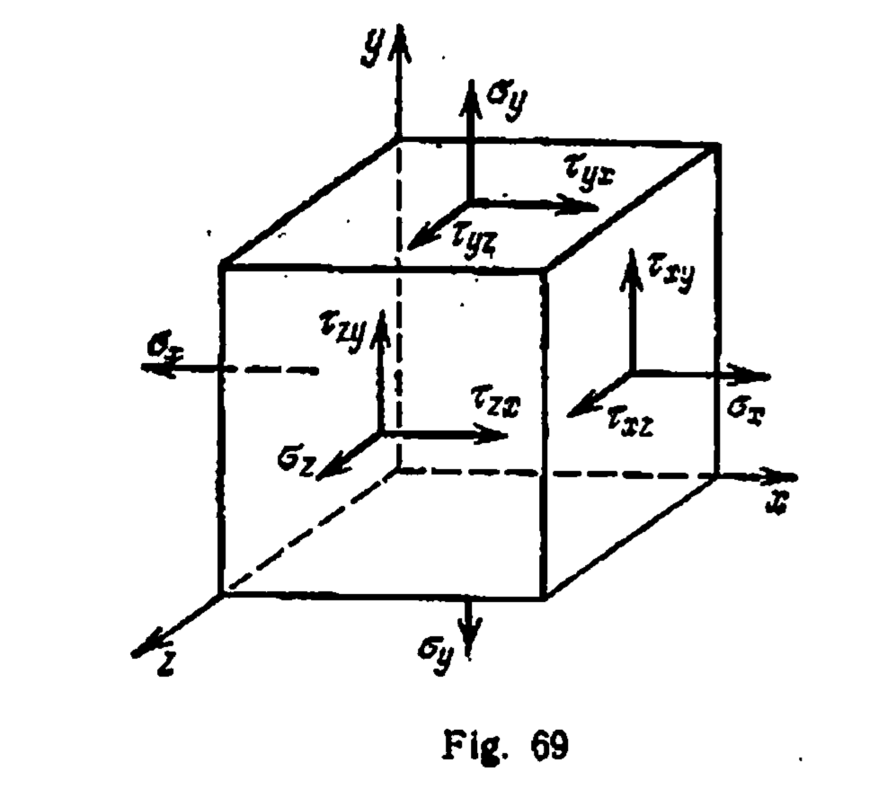
 and
and  are vectors; you can see the multiple stresses in Figure 69. We use the notation
  because the modulus of elasticity
  is a material property and thus is a part of the elasticity matrix
 ![\left[\begin{array}{cccccc} {\frac{{\it E}\,\left(1-\nu\right)}{\left(1+\nu\right)\left(1-2\,\nu\right)}} & {\frac{{\it E}\,\nu}{\left(1+\nu\right)\left(1-2\,\nu\right)}} & {\frac{{\it E}\,\nu}{\left(1+\nu\right)\left(1-2\,\nu\right)}} & 0 & 0 & 0\\ \noalign{\medskip}{\frac{{\it E}\,\nu}{\left(1+\nu\right)\left(1-2\,\nu\right)}} & {\frac{{\it E}\,\left(1-\nu\right)}{\left(1+\nu\right)\left(1-2\,\nu\right)}} & {\frac{{\it E}\,\nu}{\left(1+\nu\right)\left(1-2\,\nu\right)}} & 0 & 0 & 0\\ \noalign{\medskip}{\frac{{\it E}\,\nu}{\left(1+\nu\right)\left(1-2\,\nu\right)}} & {\frac{{\it E}\,\nu}{\left(1+\nu\right)\left(1-2\,\nu\right)}} & {\frac{{\it E}\,\left(1-\nu\right)}{\left(1+\nu\right)\left(1-2\,\nu\right)}} & 0 & 0 & 0\\ \noalign{\medskip}0 & 0 & 0 & {\frac{{\it E}\,\left(1-\nu\right)}{\left(1+\nu\right)\left(2-2\,\nu\right)}} & 0 & 0\\ \noalign{\medskip}0 & 0 & 0 & 0 & {\frac{{\it E}\,\left(1-\nu\right)}{\left(1+\nu\right)\left(2-2\,\nu\right)}} & 0\\ \noalign{\medskip}0 & 0 & 0 & 0 & 0 & {\frac{{\it E}\,\left(1-\nu\right)}{\left(1+\nu\right)\left(2-2\,\nu\right)}} \end{array}\right]\left[\begin{array}{c} \epsilon_{{x}}\\ \noalign{\medskip}\epsilon_{{y}}\\ \noalign{\medskip}\epsilon_{{z}}\\ \noalign{\medskip}\gamma{}_{{\it xy}}\\ \noalign{\medskip}{\it \gamma}_{{\it yz}}\\ \noalign{\medskip}{\it \gamma}_{{\it zx}} \end{array}\right]=\left[\begin{array}{c} \sigma_{{x}}\\ \noalign{\medskip}\sigma_{{y}}\\ \noalign{\medskip}\sigma_{{z}}\\ \noalign{\medskip}\tau_{{\it xy}}\\ \noalign{\medskip}\tau_{{\it yz}}\\ \noalign{\medskip}\tau_{{\it zx}} \end{array}\right]](https://s0.wp.com/latex.php?latex=%5Cleft%5B%5Cbegin%7Barray%7D%7Bcccccc%7D+%7B%5Cfrac%7B%7B%5Cit+E%7D%5C%2C%5Cleft%281-%5Cnu%5Cright%29%7D%7B%5Cleft%281%2B%5Cnu%5Cright%29%5Cleft%281-2%5C%2C%5Cnu%5Cright%29%7D%7D+%26+%7B%5Cfrac%7B%7B%5Cit+E%7D%5C%2C%5Cnu%7D%7B%5Cleft%281%2B%5Cnu%5Cright%29%5Cleft%281-2%5C%2C%5Cnu%5Cright%29%7D%7D+%26+%7B%5Cfrac%7B%7B%5Cit+E%7D%5C%2C%5Cnu%7D%7B%5Cleft%281%2B%5Cnu%5Cright%29%5Cleft%281-2%5C%2C%5Cnu%5Cright%29%7D%7D+%26+0+%26+0+%26+0%5C%5C+%5Cnoalign%7B%5Cmedskip%7D%7B%5Cfrac%7B%7B%5Cit+E%7D%5C%2C%5Cnu%7D%7B%5Cleft%281%2B%5Cnu%5Cright%29%5Cleft%281-2%5C%2C%5Cnu%5Cright%29%7D%7D+%26+%7B%5Cfrac%7B%7B%5Cit+E%7D%5C%2C%5Cleft%281-%5Cnu%5Cright%29%7D%7B%5Cleft%281%2B%5Cnu%5Cright%29%5Cleft%281-2%5C%2C%5Cnu%5Cright%29%7D%7D+%26+%7B%5Cfrac%7B%7B%5Cit+E%7D%5C%2C%5Cnu%7D%7B%5Cleft%281%2B%5Cnu%5Cright%29%5Cleft%281-2%5C%2C%5Cnu%5Cright%29%7D%7D+%26+0+%26+0+%26+0%5C%5C+%5Cnoalign%7B%5Cmedskip%7D%7B%5Cfrac%7B%7B%5Cit+E%7D%5C%2C%5Cnu%7D%7B%5Cleft%281%2B%5Cnu%5Cright%29%5Cleft%281-2%5C%2C%5Cnu%5Cright%29%7D%7D+%26+%7B%5Cfrac%7B%7B%5Cit+E%7D%5C%2C%5Cnu%7D%7B%5Cleft%281%2B%5Cnu%5Cright%29%5Cleft%281-2%5C%2C%5Cnu%5Cright%29%7D%7D+%26+%7B%5Cfrac%7B%7B%5Cit+E%7D%5C%2C%5Cleft%281-%5Cnu%5Cright%29%7D%7B%5Cleft%281%2B%5Cnu%5Cright%29%5Cleft%281-2%5C%2C%5Cnu%5Cright%29%7D%7D+%26+0+%26+0+%26+0%5C%5C+%5Cnoalign%7B%5Cmedskip%7D0+%26+0+%26+0+%26+%7B%5Cfrac%7B%7B%5Cit+E%7D%5C%2C%5Cleft%281-%5Cnu%5Cright%29%7D%7B%5Cleft%281%2B%5Cnu%5Cright%29%5Cleft%282-2%5C%2C%5Cnu%5Cright%29%7D%7D+%26+0+%26+0%5C%5C+%5Cnoalign%7B%5Cmedskip%7D0+%26+0+%26+0+%26+0+%26+%7B%5Cfrac%7B%7B%5Cit+E%7D%5C%2C%5Cleft%281-%5Cnu%5Cright%29%7D%7B%5Cleft%281%2B%5Cnu%5Cright%29%5Cleft%282-2%5C%2C%5Cnu%5Cright%29%7D%7D+%26+0%5C%5C+%5Cnoalign%7B%5Cmedskip%7D0+%26+0+%26+0+%26+0+%26+0+%26+%7B%5Cfrac%7B%7B%5Cit+E%7D%5C%2C%5Cleft%281-%5Cnu%5Cright%29%7D%7B%5Cleft%281%2B%5Cnu%5Cright%29%5Cleft%282-2%5C%2C%5Cnu%5Cright%29%7D%7D+%5Cend%7Barray%7D%5Cright%5D%5Cleft%5B%5Cbegin%7Barray%7D%7Bc%7D+%5Cepsilon_%7B%7Bx%7D%7D%5C%5C+%5Cnoalign%7B%5Cmedskip%7D%5Cepsilon_%7B%7By%7D%7D%5C%5C+%5Cnoalign%7B%5Cmedskip%7D%5Cepsilon_%7B%7Bz%7D%7D%5C%5C+%5Cnoalign%7B%5Cmedskip%7D%5Cgamma%7B%7D_%7B%7B%5Cit+xy%7D%7D%5C%5C+%5Cnoalign%7B%5Cmedskip%7D%7B%5Cit+%5Cgamma%7D_%7B%7B%5Cit+yz%7D%7D%5C%5C+%5Cnoalign%7B%5Cmedskip%7D%7B%5Cit+%5Cgamma%7D_%7B%7B%5Cit+zx%7D%7D+%5Cend%7Barray%7D%5Cright%5D%3D%5Cleft%5B%5Cbegin%7Barray%7D%7Bc%7D+%5Csigma_%7B%7Bx%7D%7D%5C%5C+%5Cnoalign%7B%5Cmedskip%7D%5Csigma_%7B%7By%7D%7D%5C%5C+%5Cnoalign%7B%5Cmedskip%7D%5Csigma_%7B%7Bz%7D%7D%5C%5C+%5Cnoalign%7B%5Cmedskip%7D%5Ctau_%7B%7B%5Cit+xy%7D%7D%5C%5C+%5Cnoalign%7B%5Cmedskip%7D%5Ctau_%7B%7B%5Cit+yz%7D%7D%5C%5C+%5Cnoalign%7B%5Cmedskip%7D%5Ctau_%7B%7B%5Cit+zx%7D%7D+%5Cend%7Barray%7D%5Cright%5D+&bg=ffffff&fg=777777&s=0&c=20201002) (3)
(3) (4)
(4) (5)
(5) is Poisson’s Ratio and
  is the shear modulus of elasticity. The latter is very useful in soil mechanics (
 (6)
(6) blows up (or becomes singular, as we say in polite circles) when
  . Materials where this is the case (such as very soft clays) are in reality fluids, the normal stresses become equal and the shear stresses only appear when the fluid moves. Avoiding this condition is one of the challenges of geotechnical finite element analysis.
![\left[\begin{array}{cccccc} {\frac{\left(1-\nu\right)\lambda}{\nu}} & \lambda & \lambda & 0 & 0 & 0\\ \noalign{\medskip}\lambda & {\frac{\left(1-\nu\right)\lambda}{\nu}} & \lambda & 0 & 0 & 0\\ \noalign{\medskip}\lambda & \lambda & {\frac{\left(1-\nu\right)\lambda}{\nu}} & 0 & 0 & 0\\ \noalign{\medskip}0 & 0 & 0 & G & 0 & 0\\ \noalign{\medskip}0 & 0 & 0 & 0 & G & 0\\ \noalign{\medskip}0 & 0 & 0 & 0 & 0 & G \end{array}\right] \left[\begin{array}{c} \epsilon_{{x}}\\ \noalign{\medskip}\epsilon_{{y}}\\ \noalign{\medskip}\epsilon_{{z}}\\ \noalign{\medskip}\gamma{}_{{\it xy}}\\ \noalign{\medskip}{\it \gamma}_{{\it yz}}\\ \noalign{\medskip}{\it \gamma}_{{\it zx}} \end{array}\right]=\left[\begin{array}{c} \sigma_{{x}}\\ \noalign{\medskip}\sigma_{{y}}\\ \noalign{\medskip}\sigma_{{z}}\\ \noalign{\medskip}\tau_{{\it xy}}\\ \noalign{\medskip}\tau_{{\it yz}}\\ \noalign{\medskip}\tau_{{\it zx}} \end{array}\right]](https://s0.wp.com/latex.php?latex=%5Cleft%5B%5Cbegin%7Barray%7D%7Bcccccc%7D+%7B%5Cfrac%7B%5Cleft%281-%5Cnu%5Cright%29%5Clambda%7D%7B%5Cnu%7D%7D+%26+%5Clambda+%26+%5Clambda+%26+0+%26+0+%26+0%5C%5C+%5Cnoalign%7B%5Cmedskip%7D%5Clambda+%26+%7B%5Cfrac%7B%5Cleft%281-%5Cnu%5Cright%29%5Clambda%7D%7B%5Cnu%7D%7D+%26+%5Clambda+%26+0+%26+0+%26+0%5C%5C+%5Cnoalign%7B%5Cmedskip%7D%5Clambda+%26+%5Clambda+%26+%7B%5Cfrac%7B%5Cleft%281-%5Cnu%5Cright%29%5Clambda%7D%7B%5Cnu%7D%7D+%26+0+%26+0+%26+0%5C%5C+%5Cnoalign%7B%5Cmedskip%7D0+%26+0+%26+0+%26+G+%26+0+%26+0%5C%5C+%5Cnoalign%7B%5Cmedskip%7D0+%26+0+%26+0+%26+0+%26+G+%26+0%5C%5C+%5Cnoalign%7B%5Cmedskip%7D0+%26+0+%26+0+%26+0+%26+0+%26+G+%5Cend%7Barray%7D%5Cright%5D++%5Cleft%5B%5Cbegin%7Barray%7D%7Bc%7D+%5Cepsilon_%7B%7Bx%7D%7D%5C%5C+%5Cnoalign%7B%5Cmedskip%7D%5Cepsilon_%7B%7By%7D%7D%5C%5C+%5Cnoalign%7B%5Cmedskip%7D%5Cepsilon_%7B%7Bz%7D%7D%5C%5C+%5Cnoalign%7B%5Cmedskip%7D%5Cgamma%7B%7D_%7B%7B%5Cit+xy%7D%7D%5C%5C+%5Cnoalign%7B%5Cmedskip%7D%7B%5Cit+%5Cgamma%7D_%7B%7B%5Cit+yz%7D%7D%5C%5C+%5Cnoalign%7B%5Cmedskip%7D%7B%5Cit+%5Cgamma%7D_%7B%7B%5Cit+zx%7D%7D+%5Cend%7Barray%7D%5Cright%5D%3D%5Cleft%5B%5Cbegin%7Barray%7D%7Bc%7D+%5Csigma_%7B%7Bx%7D%7D%5C%5C+%5Cnoalign%7B%5Cmedskip%7D%5Csigma_%7B%7By%7D%7D%5C%5C+%5Cnoalign%7B%5Cmedskip%7D%5Csigma_%7B%7Bz%7D%7D%5C%5C+%5Cnoalign%7B%5Cmedskip%7D%5Ctau_%7B%7B%5Cit+xy%7D%7D%5C%5C+%5Cnoalign%7B%5Cmedskip%7D%5Ctau_%7B%7B%5Cit+yz%7D%7D%5C%5C+%5Cnoalign%7B%5Cmedskip%7D%5Ctau_%7B%7B%5Cit+zx%7D%7D+%5Cend%7Barray%7D%5Cright%5D+&bg=ffffff&fg=777777&s=0&c=20201002) (7)
(7)![\left[\begin{array}{c} \sigma_{{x}}\\ \noalign{\medskip}\sigma_{{y}}\\ \noalign{\medskip}\sigma_{{z}}\\ \noalign{\medskip}\tau_{{\it xy}}\\ \noalign{\medskip}\tau_{{\it yz}}\\ \noalign{\medskip}\tau_{{\it zx}} \end{array}\right] = \left[\begin{array}{c} {\frac{\left(1-\nu\right)\lambda\,\epsilon_{{x}}}{\nu}}+\lambda\,\epsilon_{{y}}+\lambda\,\epsilon_{{z}}\\ \noalign{\medskip}\lambda\,\epsilon_{{x}}+{\frac{\left(1-\nu\right)\lambda\,\epsilon_{{y}}}{\nu}}+\lambda\,\epsilon_{{z}}\\ \noalign{\medskip}\lambda\,\epsilon_{{x}}+\lambda\,\epsilon_{{y}}+{\frac{\left(1-\nu\right)\lambda\,\epsilon_{{z}}}{\nu}}\\ \noalign{\medskip}G{\it \gamma}_{{\it xy}}\\ \noalign{\medskip}G{\it \gamma}_{{\it yz}}\\ \noalign{\medskip}G{\it \gamma}_{{\it zx}} \end{array}\right]](https://s0.wp.com/latex.php?latex=%5Cleft%5B%5Cbegin%7Barray%7D%7Bc%7D+%5Csigma_%7B%7Bx%7D%7D%5C%5C+%5Cnoalign%7B%5Cmedskip%7D%5Csigma_%7B%7By%7D%7D%5C%5C+%5Cnoalign%7B%5Cmedskip%7D%5Csigma_%7B%7Bz%7D%7D%5C%5C+%5Cnoalign%7B%5Cmedskip%7D%5Ctau_%7B%7B%5Cit+xy%7D%7D%5C%5C+%5Cnoalign%7B%5Cmedskip%7D%5Ctau_%7B%7B%5Cit+yz%7D%7D%5C%5C+%5Cnoalign%7B%5Cmedskip%7D%5Ctau_%7B%7B%5Cit+zx%7D%7D+%5Cend%7Barray%7D%5Cright%5D+%3D+%5Cleft%5B%5Cbegin%7Barray%7D%7Bc%7D+%7B%5Cfrac%7B%5Cleft%281-%5Cnu%5Cright%29%5Clambda%5C%2C%5Cepsilon_%7B%7Bx%7D%7D%7D%7B%5Cnu%7D%7D%2B%5Clambda%5C%2C%5Cepsilon_%7B%7By%7D%7D%2B%5Clambda%5C%2C%5Cepsilon_%7B%7Bz%7D%7D%5C%5C+%5Cnoalign%7B%5Cmedskip%7D%5Clambda%5C%2C%5Cepsilon_%7B%7Bx%7D%7D%2B%7B%5Cfrac%7B%5Cleft%281-%5Cnu%5Cright%29%5Clambda%5C%2C%5Cepsilon_%7B%7By%7D%7D%7D%7B%5Cnu%7D%7D%2B%5Clambda%5C%2C%5Cepsilon_%7B%7Bz%7D%7D%5C%5C+%5Cnoalign%7B%5Cmedskip%7D%5Clambda%5C%2C%5Cepsilon_%7B%7Bx%7D%7D%2B%5Clambda%5C%2C%5Cepsilon_%7B%7By%7D%7D%2B%7B%5Cfrac%7B%5Cleft%281-%5Cnu%5Cright%29%5Clambda%5C%2C%5Cepsilon_%7B%7Bz%7D%7D%7D%7B%5Cnu%7D%7D%5C%5C+%5Cnoalign%7B%5Cmedskip%7DG%7B%5Cit+%5Cgamma%7D_%7B%7B%5Cit+xy%7D%7D%5C%5C+%5Cnoalign%7B%5Cmedskip%7DG%7B%5Cit+%5Cgamma%7D_%7B%7B%5Cit+yz%7D%7D%5C%5C+%5Cnoalign%7B%5Cmedskip%7DG%7B%5Cit+%5Cgamma%7D_%7B%7B%5Cit+zx%7D%7D+%5Cend%7Barray%7D%5Cright%5D+&bg=ffffff&fg=777777&s=0&c=20201002) (8)
(8) (9)
(9)![D_{e}^{-1}=\left[\begin{array}{cccccc} -{\frac{\nu}{\lambda\,\left(-1+\nu+2\,{\nu}^{2}\right)}} & {\frac{{\nu}^{2}}{\lambda\,\left(-1+\nu+2\,{\nu}^{2}\right)}} & {\frac{{\nu}^{2}}{\lambda\,\left(-1+\nu+2\,{\nu}^{2}\right)}} & 0 & 0 & 0\\ \noalign{\medskip}{\frac{{\nu}^{2}}{\lambda\,\left(-1+\nu+2\,{\nu}^{2}\right)}} & -{\frac{\nu}{\lambda\,\left(-1+\nu+2\,{\nu}^{2}\right)}} & {\frac{{\nu}^{2}}{\lambda\,\left(-1+\nu+2\,{\nu}^{2}\right)}} & 0 & 0 & 0\\ \noalign{\medskip}{\frac{{\nu}^{2}}{\lambda\,\left(-1+\nu+2\,{\nu}^{2}\right)}} & {\frac{{\nu}^{2}}{\lambda\,\left(-1+\nu+2\,{\nu}^{2}\right)}} & -{\frac{\nu}{\lambda\,\left(-1+\nu+2\,{\nu}^{2}\right)}} & 0 & 0 & 0\\ \noalign{\medskip}0 & 0 & 0 & {G}^{-1} & 0 & 0\\ \noalign{\medskip}0 & 0 & 0 & 0 & {G}^{-1} & 0\\ \noalign{\medskip}0 & 0 & 0 & 0 & 0 & {G}^{-1} \end{array}\right]](https://s0.wp.com/latex.php?latex=D_%7Be%7D%5E%7B-1%7D%3D%5Cleft%5B%5Cbegin%7Barray%7D%7Bcccccc%7D+-%7B%5Cfrac%7B%5Cnu%7D%7B%5Clambda%5C%2C%5Cleft%28-1%2B%5Cnu%2B2%5C%2C%7B%5Cnu%7D%5E%7B2%7D%5Cright%29%7D%7D+%26+%7B%5Cfrac%7B%7B%5Cnu%7D%5E%7B2%7D%7D%7B%5Clambda%5C%2C%5Cleft%28-1%2B%5Cnu%2B2%5C%2C%7B%5Cnu%7D%5E%7B2%7D%5Cright%29%7D%7D+%26+%7B%5Cfrac%7B%7B%5Cnu%7D%5E%7B2%7D%7D%7B%5Clambda%5C%2C%5Cleft%28-1%2B%5Cnu%2B2%5C%2C%7B%5Cnu%7D%5E%7B2%7D%5Cright%29%7D%7D+%26+0+%26+0+%26+0%5C%5C+%5Cnoalign%7B%5Cmedskip%7D%7B%5Cfrac%7B%7B%5Cnu%7D%5E%7B2%7D%7D%7B%5Clambda%5C%2C%5Cleft%28-1%2B%5Cnu%2B2%5C%2C%7B%5Cnu%7D%5E%7B2%7D%5Cright%29%7D%7D+%26+-%7B%5Cfrac%7B%5Cnu%7D%7B%5Clambda%5C%2C%5Cleft%28-1%2B%5Cnu%2B2%5C%2C%7B%5Cnu%7D%5E%7B2%7D%5Cright%29%7D%7D+%26+%7B%5Cfrac%7B%7B%5Cnu%7D%5E%7B2%7D%7D%7B%5Clambda%5C%2C%5Cleft%28-1%2B%5Cnu%2B2%5C%2C%7B%5Cnu%7D%5E%7B2%7D%5Cright%29%7D%7D+%26+0+%26+0+%26+0%5C%5C+%5Cnoalign%7B%5Cmedskip%7D%7B%5Cfrac%7B%7B%5Cnu%7D%5E%7B2%7D%7D%7B%5Clambda%5C%2C%5Cleft%28-1%2B%5Cnu%2B2%5C%2C%7B%5Cnu%7D%5E%7B2%7D%5Cright%29%7D%7D+%26+%7B%5Cfrac%7B%7B%5Cnu%7D%5E%7B2%7D%7D%7B%5Clambda%5C%2C%5Cleft%28-1%2B%5Cnu%2B2%5C%2C%7B%5Cnu%7D%5E%7B2%7D%5Cright%29%7D%7D+%26+-%7B%5Cfrac%7B%5Cnu%7D%7B%5Clambda%5C%2C%5Cleft%28-1%2B%5Cnu%2B2%5C%2C%7B%5Cnu%7D%5E%7B2%7D%5Cright%29%7D%7D+%26+0+%26+0+%26+0%5C%5C+%5Cnoalign%7B%5Cmedskip%7D0+%26+0+%26+0+%26+%7BG%7D%5E%7B-1%7D+%26+0+%26+0%5C%5C+%5Cnoalign%7B%5Cmedskip%7D0+%26+0+%26+0+%26+0+%26+%7BG%7D%5E%7B-1%7D+%26+0%5C%5C+%5Cnoalign%7B%5Cmedskip%7D0+%26+0+%26+0+%26+0+%26+0+%26+%7BG%7D%5E%7B-1%7D+%5Cend%7Barray%7D%5Cright%5D+&bg=ffffff&fg=777777&s=0&c=20201002) (10)
(10)![\left[\begin{array}{c} \epsilon_{{x}}\\ \noalign{\medskip}\epsilon_{{y}}\\ \noalign{\medskip}\epsilon_{{z}}\\ \noalign{\medskip}\gamma{}_{{\it xy}}\\ \noalign{\medskip}{\it \gamma}_{{\it yz}}\\ \noalign{\medskip}{\it \gamma}_{{\it zx}} \end{array}\right] = \left[\begin{array}{c} -{\frac{\nu\,\sigma_{{x}}}{\lambda\,\left(-1+\nu+2\,{\nu}^{2}\right)}}+{\frac{{\nu}^{2}\sigma_{{y}}}{\lambda\,\left(-1+\nu+2\,{\nu}^{2}\right)}}+{\frac{{\nu}^{2}\sigma_{{z}}}{\lambda\,\left(-1+\nu+2\,{\nu}^{2}\right)}}\\ \noalign{\medskip}{\frac{{\nu}^{2}\sigma_{{x}}}{\lambda\,\left(-1+\nu+2\,{\nu}^{2}\right)}}-{\frac{\nu\,\sigma_{{y}}}{\lambda\,\left(-1+\nu+2\,{\nu}^{2}\right)}}+{\frac{{\nu}^{2}\sigma_{{z}}}{\lambda\,\left(-1+\nu+2\,{\nu}^{2}\right)}}\\ \noalign{\medskip}{\frac{{\nu}^{2}\sigma_{{x}}}{\lambda\,\left(-1+\nu+2\,{\nu}^{2}\right)}}+{\frac{{\nu}^{2}\sigma_{{y}}}{\lambda\,\left(-1+\nu+2\,{\nu}^{2}\right)}}-{\frac{\nu\,\sigma_{{z}}}{\lambda\,\left(-1+\nu+2\,{\nu}^{2}\right)}}\\ \noalign{\medskip}{\frac{\tau_{{\it xy}}}{G}}\\ \noalign{\medskip}{\frac{\tau_{{\it yz}}}{G}}\\ \noalign{\medskip}{\frac{\tau_{{\it zx}}}{G}} \end{array}\right]](https://s0.wp.com/latex.php?latex=%5Cleft%5B%5Cbegin%7Barray%7D%7Bc%7D+%5Cepsilon_%7B%7Bx%7D%7D%5C%5C+%5Cnoalign%7B%5Cmedskip%7D%5Cepsilon_%7B%7By%7D%7D%5C%5C+%5Cnoalign%7B%5Cmedskip%7D%5Cepsilon_%7B%7Bz%7D%7D%5C%5C+%5Cnoalign%7B%5Cmedskip%7D%5Cgamma%7B%7D_%7B%7B%5Cit+xy%7D%7D%5C%5C+%5Cnoalign%7B%5Cmedskip%7D%7B%5Cit+%5Cgamma%7D_%7B%7B%5Cit+yz%7D%7D%5C%5C+%5Cnoalign%7B%5Cmedskip%7D%7B%5Cit+%5Cgamma%7D_%7B%7B%5Cit+zx%7D%7D+%5Cend%7Barray%7D%5Cright%5D+%3D+%5Cleft%5B%5Cbegin%7Barray%7D%7Bc%7D+-%7B%5Cfrac%7B%5Cnu%5C%2C%5Csigma_%7B%7Bx%7D%7D%7D%7B%5Clambda%5C%2C%5Cleft%28-1%2B%5Cnu%2B2%5C%2C%7B%5Cnu%7D%5E%7B2%7D%5Cright%29%7D%7D%2B%7B%5Cfrac%7B%7B%5Cnu%7D%5E%7B2%7D%5Csigma_%7B%7By%7D%7D%7D%7B%5Clambda%5C%2C%5Cleft%28-1%2B%5Cnu%2B2%5C%2C%7B%5Cnu%7D%5E%7B2%7D%5Cright%29%7D%7D%2B%7B%5Cfrac%7B%7B%5Cnu%7D%5E%7B2%7D%5Csigma_%7B%7Bz%7D%7D%7D%7B%5Clambda%5C%2C%5Cleft%28-1%2B%5Cnu%2B2%5C%2C%7B%5Cnu%7D%5E%7B2%7D%5Cright%29%7D%7D%5C%5C+%5Cnoalign%7B%5Cmedskip%7D%7B%5Cfrac%7B%7B%5Cnu%7D%5E%7B2%7D%5Csigma_%7B%7Bx%7D%7D%7D%7B%5Clambda%5C%2C%5Cleft%28-1%2B%5Cnu%2B2%5C%2C%7B%5Cnu%7D%5E%7B2%7D%5Cright%29%7D%7D-%7B%5Cfrac%7B%5Cnu%5C%2C%5Csigma_%7B%7By%7D%7D%7D%7B%5Clambda%5C%2C%5Cleft%28-1%2B%5Cnu%2B2%5C%2C%7B%5Cnu%7D%5E%7B2%7D%5Cright%29%7D%7D%2B%7B%5Cfrac%7B%7B%5Cnu%7D%5E%7B2%7D%5Csigma_%7B%7Bz%7D%7D%7D%7B%5Clambda%5C%2C%5Cleft%28-1%2B%5Cnu%2B2%5C%2C%7B%5Cnu%7D%5E%7B2%7D%5Cright%29%7D%7D%5C%5C+%5Cnoalign%7B%5Cmedskip%7D%7B%5Cfrac%7B%7B%5Cnu%7D%5E%7B2%7D%5Csigma_%7B%7Bx%7D%7D%7D%7B%5Clambda%5C%2C%5Cleft%28-1%2B%5Cnu%2B2%5C%2C%7B%5Cnu%7D%5E%7B2%7D%5Cright%29%7D%7D%2B%7B%5Cfrac%7B%7B%5Cnu%7D%5E%7B2%7D%5Csigma_%7B%7By%7D%7D%7D%7B%5Clambda%5C%2C%5Cleft%28-1%2B%5Cnu%2B2%5C%2C%7B%5Cnu%7D%5E%7B2%7D%5Cright%29%7D%7D-%7B%5Cfrac%7B%5Cnu%5C%2C%5Csigma_%7B%7Bz%7D%7D%7D%7B%5Clambda%5C%2C%5Cleft%28-1%2B%5Cnu%2B2%5C%2C%7B%5Cnu%7D%5E%7B2%7D%5Cright%29%7D%7D%5C%5C+%5Cnoalign%7B%5Cmedskip%7D%7B%5Cfrac%7B%5Ctau_%7B%7B%5Cit+xy%7D%7D%7D%7BG%7D%7D%5C%5C+%5Cnoalign%7B%5Cmedskip%7D%7B%5Cfrac%7B%5Ctau_%7B%7B%5Cit+yz%7D%7D%7D%7BG%7D%7D%5C%5C+%5Cnoalign%7B%5Cmedskip%7D%7B%5Cfrac%7B%5Ctau_%7B%7B%5Cit+zx%7D%7D%7D%7BG%7D%7D+%5Cend%7Barray%7D%5Cright%5D++&bg=ffffff&fg=777777&s=0&c=20201002) (11)
(11)