
Students and practicioners of soil mechanics alike are used to seeing triaxial test results that look like this (from DM 7.01):

Ideally, the Mohr-Coulomb failure line should be straight, but with real soils it doesn’t have to be that way. With the advent of finite element analysis we also have the failure function to consider, thus (from Warrington (2016)):

All of these involve constructing (or using) a line which is tangent to a circle at failure. This can be confusing to understand completely. The biggest problem from a “newbie” standpoint is that the maximum shear defined by the circle of stress (its radius) and the failure shear stress defined by the intersection of the circle with the Mohr-Coulomb failure envelope are not the same.
Is there a better graphical way to represent the interaction of stresses with the Mohr-Coulomb failure criterion? The answer is “yes” and it involves the use of p-q diagrams. These have been around for a long time and are used in such things as critical state soil mechanics and stress paths. A broad explanation of these is found in our new publication, Geotechnical Site Characterization. The purpose of this article is to present these as a purely mathematical transformation of the classic Mohr-Coulomb diagram. This is especially important since their explanation is frequently lacking in textbooks.
The Basics
Consider the failure function, which is valid throughout the Mohr-Coulomb plot. It can be stated as follows:

(The main difference between the two formulations is multiplication by 2; the failure function can either be diametral or radial relative to Mohr’s Circle. With a purely elasto-plastic model, the results are the same.)
Now let us define the following terms:


We should also define the following:

The physical significance of the last one is discussed in this post. In any case we can start with 


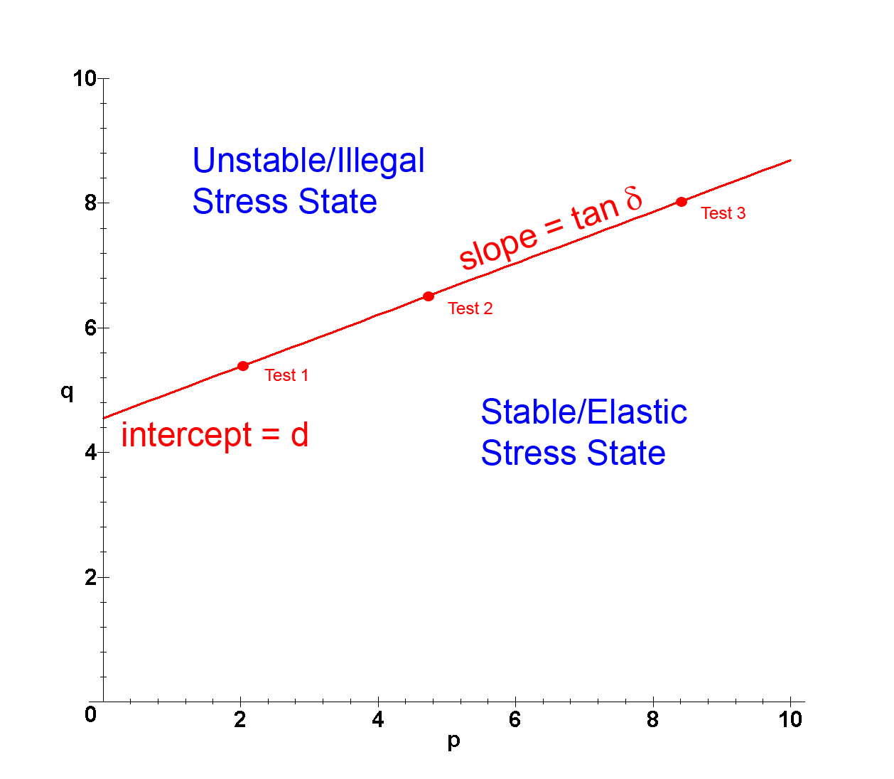
For the failure line, 


This is a classic “slope-intercept” form like 


Some Observations
- For the case of a purely cohesive soil, where
, the failure envelope is horizontal, just like with a conventional Mohr-Coulomb diagram.
- For the case of a purely cohesionless soil, where
, the y-intercept is in both cases through the origin.
- The two diagrams are thus very similar visually, it’s just that the p-q diagram eliminates the circles and tangents, reducing each case to a single point.
Examples of Use
Drained Triaxial Test in Clay
Consider the example of a drained triaxial test in clay with the following two data points:
- Confining Pressure = 70 kPa; Failure Pressure = 200 kPa.
- Confining Pressure = 160 kPa; Failure Pressure = 383.5 kPa.
Determine the friction angle and cohesion using the p-q diagram.
We first start by computing p and q for each case as follows:


The slope is simply

from which


Use of this method eliminates the need to solve two equations in two unknowns, and the repetition of the quantity 

Example from Soils in Construction
Another example of this comes from the textbook Soils in Construction. Things are a little trickier because of the book’s notation but we’ll work through that.
Consider a two-triaxial test result as follows:
- p1 = 295 kPa, p3 = 20 kPa
- p1 = 329 kPa, p3 = 40 kPa
The problem here is immediately apparent: Soils in Construction uses p as its variable for soil pressures and stresses. We’ll get around the subscript issue by designating the two p and q values as a and b respectively.
That disposed of, we can compute these as follows:


The slope is simply

from which


Although there are several steps, there is no need to solve two equations simultaneously, as is the case in the book.
Stress Paths
As mentioned earlier, p-q diagrams are commonly used with stress paths. An example of this from DM 7.01 is shown below.

We note that p and q are defined here exactly as we have them above. (That isn’t always the case; examples of other formulations of the p-q diagram are here. We should note, however, that for this diagram 
As an example, consider the stress path example from Verruijt, A., and van Bars, S. (2007). Soil Mechanics. VSSD, Delft, the Netherlands. The basic data from Test 1 are below:
 | Deviator Stress | Pore Water Pressure |
| 40 | 0 | 0 |
| 40 | 10 | 4 |
| 40 | 20 | 9 |
| 40 | 30 | 13 |
| 40 | 40 | 17 |
| 40 | 50 | 21 |
| 40 | 60 | 25 |
Using the p-q diagram and performing some calculations (which are shown in the spreadsheet Stress Paths Verruijt Example) the stress paths can be plotted as follows:
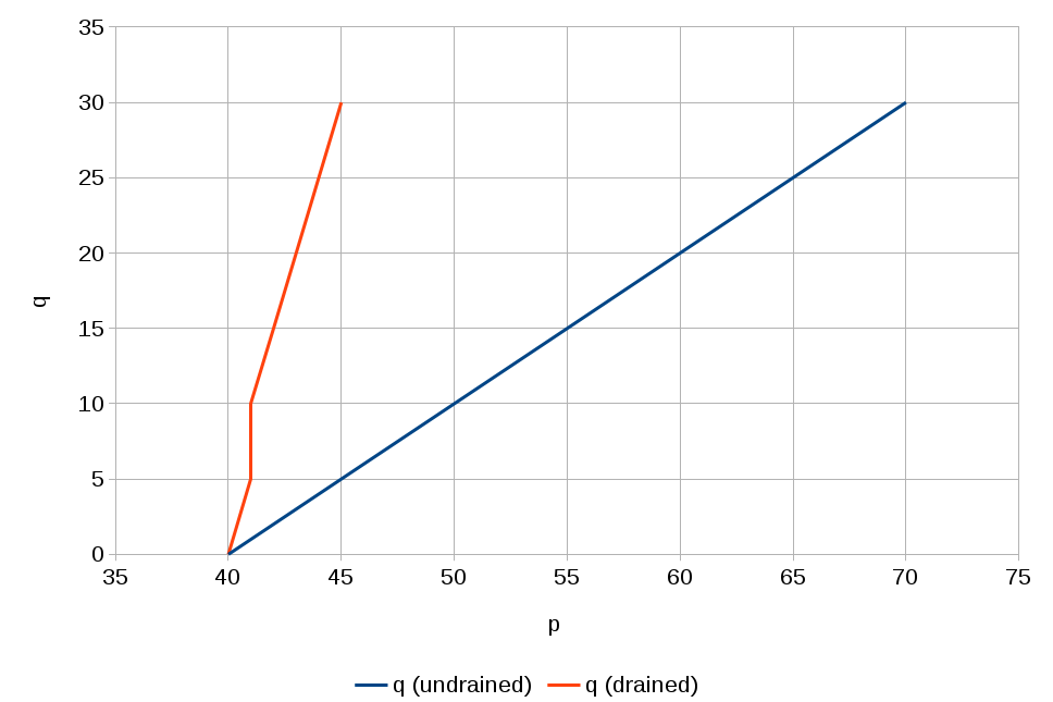
It’s worth noting that the q axis is unaffected by the drainage condition because the pore water pressures cancel each other out. Only the p-axis changes.
Conclusion
The p-q diagram is a method of simplifying the analysis of triaxial and other stress data which are commonly used in soil mechanics. It can be used in a variety of applications and solve a range of problems.
 (1)
(1) is the pore water pressure,
  is the unit weight of the water, and
  is the distance from the phreatic surface/water table, where by definition
  .
. (2)
(2) is the change in the pore water pressure from some elevation 1 in the soil to some other elevation 2 in the soil, and
  is the change in elevation from point 1 to point 2. As a condition, since
  (3)
(3)
 can be computed using methods described in

 (4)
(4) , and thus
  .
. (5)
(5) (6)
(6) (7)
(7) .
. . Keeping in mind that positive z is downwards, we start from the top of the soil sample. The change in pore water pressure from the surface is
 (8)
(8) (9)
(9)

 (10)
(10) cannot be applied directly. The reason is simple: even with moving water, the direct hydrostatic effect due to gravity does not go away, and has to be considered. Thus we have the term
  rather than just
  .
. (11)
(11) yields
 (12)
(12)

