Part of Soils in Construction‘s presentation of dewatering is this topic. I cover it in my treatment of flow nets in Soil Mechanics: Groundwater and Permeability II; however, Soils in Construction uses a less computationally intensive approach. In this piece I’ll explain that, give some better graphics than the book had available at the time of publication, and compare them with the flow net/FEA results I discussed in my Soil Mechanics course.
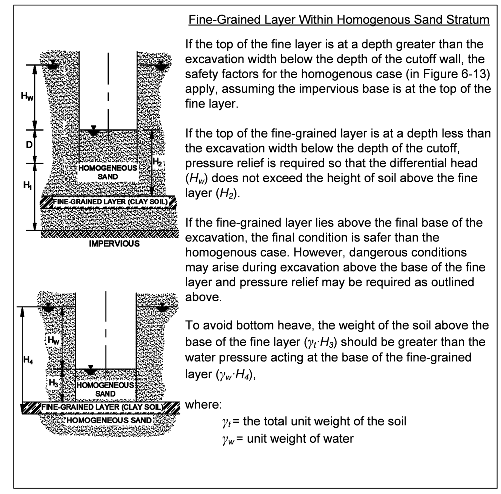
Let us consider the problem of a braced cut, which is commonly used for “cut and cover” construction. Such a construction is shown at the right. One of the challenges of temporary works such as this is to insure that a) there is sufficient pumping capacity to keep the “steel trench” dry, and b) the hydraulic gradient of the water coming up into the trench is sufficiently low to avoid soil boiling and bottom heave due to that soil boiling. (Bottom heave can take place due to other factors as well.) An example of that (showing a flow net) is below to the left.
Because the cut is internally braced, it is usually possible to make the sheeting walls simply penetrate to just below the bottom of the trench. However, in order to mitigate the effects of water flowing from around the cut into the bottom, the sheeting can be extended. The idea is that, the longer the extensions, the longer distance the water has to flow, the increased resistance of the soil to flow, and the lower the hydraulic gradients, which both reduce the flow overall and the possibility that the soil at the bottom of the trench will boil, i.e., enter into a quick condition.
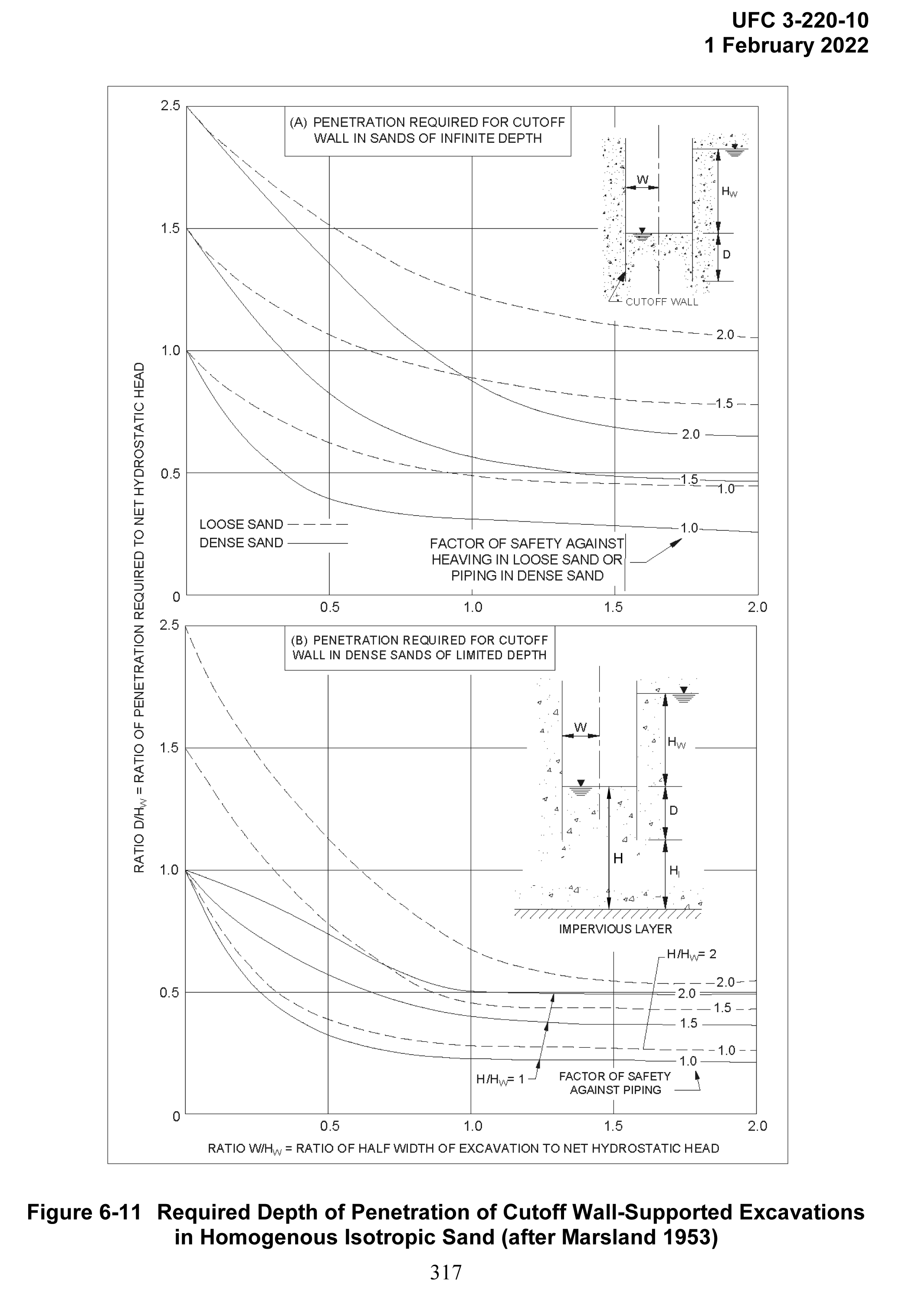
Charts to determine the minimum extension of the sheeting. These were developed by Marsland (1953). In the book they were taken from NAVFAC DM 7.01, but since the book’s publication NAVFAC DM 7.1 has redone the graphics, and you can see that below (and click on it to download). It is important to note that there is an error in the lower part of this figure; I checked it against Marsland (1953) and have modified it a bit to restore it to Marsland’s original formulation, the following example will show how it is supposed to be used.
Impervious layer 20’ below the toe of the sheeting
Length of Sheet Piling = 66’
Water table at the excavation level on the excavation side
Water table 6’ below the top of the sheeting on the soil side
Variables for chart above
Hw = 38 – 6 = 32′
D = 66 – 38 = 28′
Hl = 20′
H = D + Hl = 28 + 20 = 48′
W = 16′
Even though the graphic for the problem doesn’t show it, the problem statement indicates an impervious layer below the excavation; thus, we will use the lower chart for this problem.
Soil Conditions
Uniform medium sand, k = 0.0003 ft/sec
Saturated Unit Weight = 115 pcf
We need to, one way or another, insure that the design does not experience soil boiling.
The “rule of thumb” in Soils in Construction states that “the depth of penetration of the cut-off wall below the bottom of the excavation should be a third of the “length” computed. For this wall, the ratio is 28/66 = 42%, which means the rule of thumb is achieved.
Turning to the chart above, we must compute three quantities:
The x-axis ratio of half width of excavation to net hydrostatic head, or W/Hw = 16/32 = 0.5;
the y-axis ratio of penetration required to net hydrostatic head, or D/Hw = 28/32 = 0.875; and
the ratio of the depth between the bottom of the excavation and the impervious layer to the net hydrostatic head, or H/Hw = 48/32 = 1.5.
In this case we only have two values of H/Hw to work with: 1 and 2. For H/Hw = 1, FS ~ 2.5 (this is a very rough extrapolation.) For H/Hw = 2, FS = 1.75. Since H/Hw = 1.5 is in the middle between the two, the FS = (2.5+1.75)/2 = 2.125.
If we want to check our results by neglecting the impervious layer, we use the upper chart, and assuming the soil is closer to being a loose sand, FS ~ 1.4.
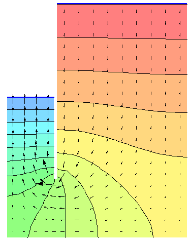
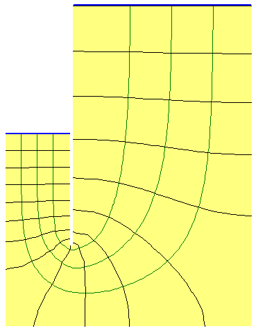
So how does this all compare to a flow net/FEA result? Same is given below.
At the right is a flow net generated by the finite element program SEEP-W. At the left is a chart showing the direction of the water flow (arrows) and the hydraulic head (coloured bands.) An in-depth explanation of these can be found at Soil Mechanics: Groundwater and Permeability II. The results are as follows:
The factor of safety from the chart ignoring the presence of the impervious layer is the closest to the FEA/flow net result. For the chart with the impervious layer, the extrapolation for the lower factor of safety should perhaps be ignored.
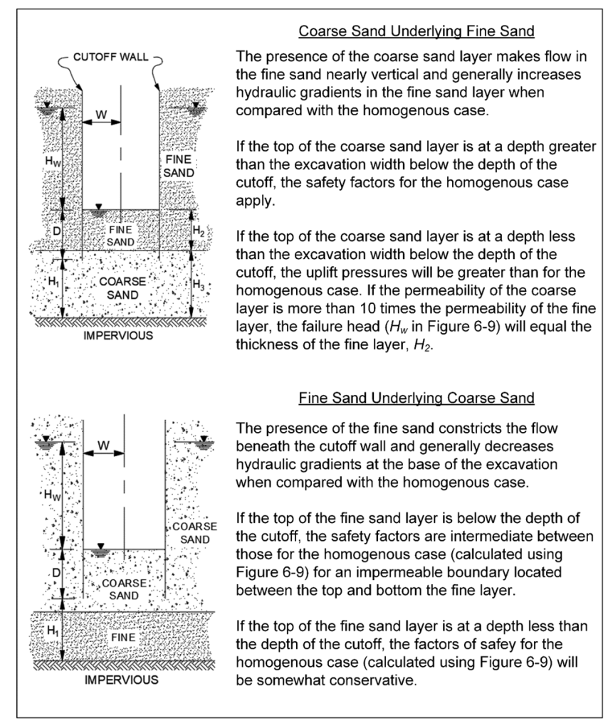
A couple of other charts (based on Marsland (1953)) are shown below.
References
Marsland, A.R. 1953. “Model Experiments to Study the Influence of Seepage on the Stability of a Sheeted Excavation in Sand.” Geotechnique, 3(6), 223-241.
Last year I posted The Sorry State of Compression Coefficients where I a) gave a brief summary of earlier posts on consolidation settlement and b)showed that there was more than one way to express them. An example of the “alternative” (for geotechs in some countries it’s the accepted way) compression coefficient is “Hough’s Method” which is featured in both the Soils and Foundations Reference Manual and the Shallow Foundations manual. Hough’s Method, however, is for cohesionless soils. Why, you ask, can methods usually associated with cohesive soils be applied to cohesionless ones? Because consolidation settlement methods using the logarithmic difference of pressure reflect the fact that the elastic (or shear) modulus of a soil increases as the void ratio/porosity of the material decreases, which I discuss in From Elasticity to Consolidation Settlement: Resolving the Issue of Jean-Louis Briaud’s “Pet Peeve”.
In this post I will attempt to do two things:
The method as presented in the above references has been described as too conservative, i.e., the settlements predicted are too large. I will attempt to explain this and perhaps offer a solution based on Hough’s own works.
Discuss the whole business of bearing capacity vs. settlement failure in shallow foundations, which was perhaps the greatest legacy of Hough’s work and remains an important issue in geotechnical engineering today.
Bearing Capacity vs. Settlement
Terzaghi’s solution (or more accurately his adaptation of Prandtl’s punching shear theory) of the bearing capacity problems was one in a number of solutions that became “reference standard” in geotechnical engineering.
We were regaled with photos of Canadian grain elevators on their side to show that bearing capacity failure was the first thing we should look for in shallow foundation design. Terzaghi’s formula was so highly regarded that for many years it was fashionable for introductory geotechnical courses to require students to learn both Terzaghi’s method and the subsequent improvements/extensions of that method by researchers such as Meyerhof, Vesic, Brinch Hansen, etc..
Up until that time shallow foundations were generally designed using what we call “presumptive bearing capacities” based on soil types and foundation configurations. These were enshrined in the building codes of the day. They were generally purely empirical in nature, as was most of geotech in the era before Terzaghi and his contemporaries. They had one advantage however: because they were derived from actual performance, be it ever so crude, they included the effects of soil settlement under load.
Like any other engineering material, only on a larger basis (because their elastic/shear moduli were several orders of magnitude lower than more conventional materials) soil is deformable under load. That deformation not only allows the foundation to deflect under load, it also affects the failure surfaces as they develop. The latter reality became apparent and so we have the modification of the bearing capacity for punching and local shear. It should be noted that Terzaghi and Peck were well aware of the problem of settlement, and included provision for it in their classic 1948 textbook Soil Mechanics in Engineering Practice.
One possible solution was to use elastic theory for the initial settlement. The implementation of that is discussed in Analytical Boussinesq Solutions for Strip, Square and Rectangular Loads. It is even possible to develop a lower bound solution for the bearing capacity problem, as was discussed in Lower and Upper Bound Solutions for Bearing Capacity. The problem with this is twofold. The first is that the lower bound solution assumes that the footing is a purely flexible foundation, which is not really true with this type of foundation. The second is that, if we went to the other extreme and assumed a purely rigid foundation, by elastic theory the stresses at the corners is infinite for any load. (This is conventionally attributed to foundations in cohesive soil, but it can be shown to be true by elastic theory.)
Hough’s Settlement Method
Hough presented his settlement method in his 1959 ASCE paper. He starts by presenting a graph similar to the following, which illustrates the transition from small, elastic displacement to large inelastic ones:
The solution is in the form (similar to that presented in Verruijt) of
The coefficient is determined using a chart which is below.
The chart itself is basically the same as the one in Hough (1959,) but now things get complicated.
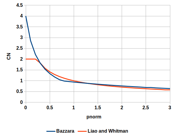
Cheney and Chassie (2000) recommend that the SPT blowcounts be corrected for overburden pressure before correlating the N-values to the bearing capacity index, C′. An overburden correction by Bazaraa (1967) was recommended by Cheney and Chassie (2000). Since that time, many researchers have studied the effect of overburden stress on the SPT N-value, largely in support of liquefaction hazard assessment procedures. Recent consensus by the 1996 and 1998 National Center for Earthquake Engineering Research (NCEER) (Youd et al., 2001) concluded that the correction proposed by Liao & Whitman (1986) (shown in Figure 5-18) could be used for routine engineering applications. Therefore, the correction by Liao & Whitman is included here as part of the Hough procedure, in particular because it is easy to calculate and can be used without charts in simple computation spreadsheets.
The basic problem with this is that Hough himself never mentions any kind of correction for the variations of the SPT tests, overburden or otherwise, and that in modifying Hough’s Method we run the risk of making some assumptions that may not be applicable.
The idea of using the SPT tests, even with shallow foundations in cohesionless soils such as the ones Hough is concerned about, is admirable on the face because undisturbed samples of these soils are hard to obtain in normal soil testing. The problem with SPT tests–which were coming into acceptance when Hough presented his original method–is that their variations in both configuration and those induced by the overburden are significant. It wasn’t until the 1980’s that this was “formally” sorted out with the correction system that we have today.
With our current method we have two stages of correction. The first stage is for variations in the configuration of the split spoon, the effect of the rod and borehole, and most importantly the efficiency of the hammer itself. The second is for the overburden. In both his original paper and the presentation of the method in the Second Edition of his textbook Basic Soils Engineering (1969,) Hough does not delve into either of these.
The whole point of the N60 correction (the first series) was to harmonise the results to a single mechanical standard, and one that was generally attained “back in the day” so that empirical methods such as Hough’s could be used today. We could assume that Hough’s value are at least N60 values, although we’re not guaranteed of that due to the lack of supporting data.
The business of overburden correction brings up Bazaraa (1967.) At this point credit needs to be given where credit is due: Bazaraa had the thankless task of sorting out the settlement methods which were current in his day, and that task included dealing with the variations of the SPT method. Since his overburden correction method was originally used with Hough’s Method and then changed, let us compare the two. We start be defining
The two correction factors for overburden are shown below.
Except for the region where Liao and Whitman is “flat topped” the two are reasonably close, and so substituting Liao and Whitman’s correction is legitimate, assuming it should be used at all.
It should be noted, however, that Bazaraa’s objective is not to correct Hough’s method, which he did not do: it was to provide a new method of estimating settlements in cohesionless soils, and to advance Terzaghi and Peck’s 1948 method. So we are still “up in the air” about how to apply all of this to Hough’s Method.
If the overburden stress is less than the standard atmospheric pressure (approx. 2 ksf) then the N value used will be increased, the C’ values will likewise increase, and the estimated settlement will decrease, which may be more accurate but moves away from conservatism. If the opposite is true then the result will be more conservative. For shallow foundations such as Hough’s Method the lower overburden stresses will be more of a factor (depending upon the depth D.) At this point it is not clear to me (at least) that including an overburden correction is really significant given the other unsolved problems that exist with this method.
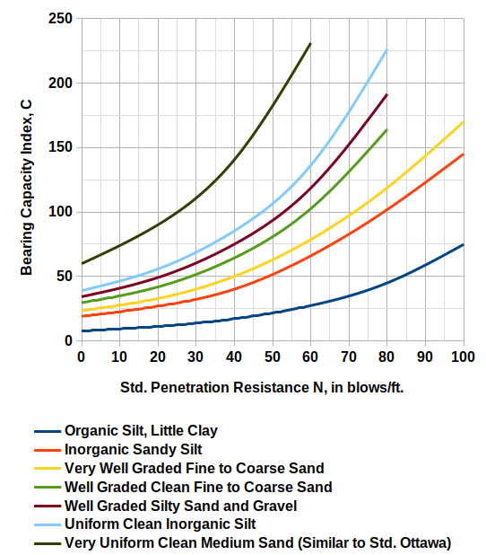
One further complicating factor is that, in the aforementioned Second Edition of Basic Soils Engineering, Hough presents a new chart (again with no explanation of correction of any kind) which is redrawn as follows:
Very Uniform Clean Medium Sand (Similar to Std. Ottawa)
58.66
0.0225
It should be noted that, where the curves are directly comparable with Hough (1959), they tend to be lower, i.e., the values of C are less. This would increase settlement and thus conservatism. At this point perhaps we should consider Hough’s Methods in the plural rather than the singular.
We have the conventional Cc based on either liquid limit, initial void ratio or water content. Hough is represented here as well; however, these correlations are for cohesive soils. Hough himself had a broader application for these.
In the Second Edition of Basic Soils Engineering, he presents a function to compute Cc as follows:
He also establishes a relationship between correlations based on liquid limit and those on void ratio, but getting to that is for another time.
In any case he presents values for this equation which are tabulated below, and include both cohesionless and cohesive soils.
a
b*
Uniform cohesionless Material (Cu < 2)
Clean Gravel
0.05
0.5
Coarse Sand
0.06
Medium Sand
0.07
Fine Sand
0.08
Inorganic Silt
0.1
Well-graded, cohesionless soil
Silty sand and gravel
0.09
0.2
Clean, coarse to fine sand
0.12
0.35
Coarse to fine silty sand
0.15
0.25
Sandy silt (inorganic)
0.18
0.25
Inorganic, cohesive soil
Silt, some clay; silty clay; clay
0.29
0.27
Organic, fine-grained soil
Organic silt, little clay
0.35
0.5
*The value of the constant b should be taken as emin whenever the latter is known or can conveniently be determined. Otherwise, use tabulated values as a rough estimate.
From here we can use the well-tried “Cc” formulae (which would include preconsolidated soils) to estimate settlement. This opens up a new vista for using conventional consolidation settlement theory to estimate the settlements of cohesionless soils.
To return to our original objectives, settlement and bearing capacity are, in the process of failure, two sides of the same thing. It is also worth noting that most foundations fail in settlement, although the failure isn’t as “spectacular” as bearing capacity.
The only way to treat them together is to use a method that can combines both phenomena, and finite element methods are capable of doing that. However our profession has been uncomfortable with “black box” methods such as these, although they really apply the same laws we use to formulate closed form solutions. In that respect they have value, and to apply methods such as Hough’s to cohesionless soils with better calibration of the constants would be a good step forward.
References
Bazaraa, A.R.S. (1967). “Use of the Standard Penetration Test for Estimating Settlements of Shallow Foundations on Sand,” Ph.D. Thesis presented to University of Illinois, Urbana.
Hough, B.K. (1959). “Compressibilty as the Basis for Soil Bearing Value,” Journal of the Soil Mechanics and Foundations Division, ASCE, Vol. 85, Part 2.
Hough, B.K. (1969). Basic Soils Engineering. Second Edition. New York: Ronald Press Company.


 is determined using a chart which is below.
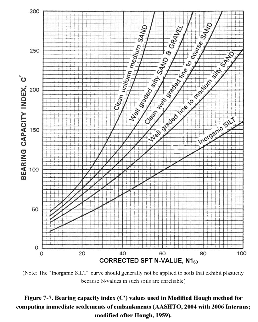

 for overburden are shown below.