books – vulcanhammer.net

Academic Issues, Geotechnical Engineering, Soil Mechanics

SLOPE Stability Software Program

Posted on 22 August 2026 by Don Warrington

Ever since this site’s predecessor was started in 1997, one of the things it’s “about” is offering useful documents and software at no charge. With software that’s become more difficult as operating systems have changed and some software has become inoperable on newer computer systems. We’ve gotten around that for DOS and Windows 3.1 applications, as shown in Partying Like It’s 1987: Running WEAP87 and SPILE (and other programs) on DOSBox. In this case we’re featuring a Windows-based, 32-bit software program for slope stability called–wait for it–SLOPE. It was developed by the late Arnold Verruijt, whose Soil Mechanics book I used for many years.

Downloading the Software

That’s pretty straightforward: click on the link below and save the file to your computer.

Download SLOPE Stability Software

What you’ll see is slope.zip. Computers and file download sites are getting nervous about raw Windows .exe files, so all you need to do is to extract the one and only slope.exe file from the archive.

Starting SLOPE

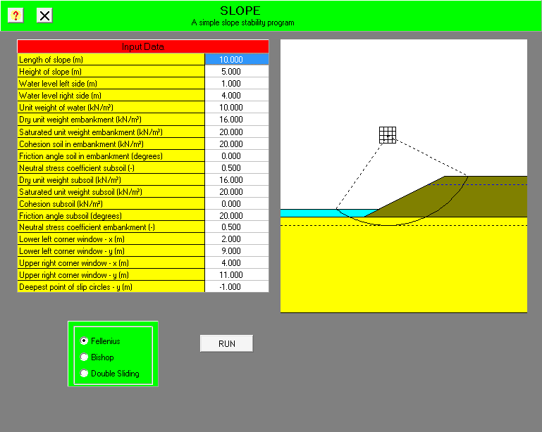
Now we come to the first discovery: slope.exe isn’t a program installation file, it is the program! You just double click on it and you will be greeted with the interface shown at the top of the post. The data entry is in the while column under “Input Data.” We will explain the input in an example.

The Example

The example is shown below, it is taken from the Soils and Foundations Reference Manual. The description from there is as follows:

Figure 6-20 shows a 35 ft high slope with a grade of 1.5H:1V. The soil properties within the slope and under it are shown on the figure. Groundwater is immediately under the slope. Calculate the factor of safety for a toe circle by using total stress analysis based on the soil properties shown.

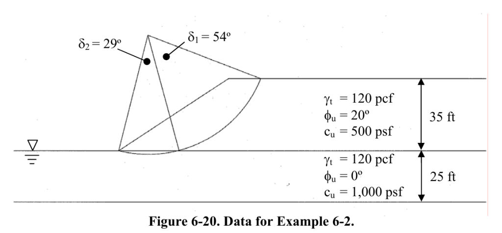
Because slope locates the slip circle of failure, we can ignore the geometry specified in that part of the drawing.

Basic Principle of Operation

SLOPE is based on classical slope stability techniques that goes back to Wolmar Fellenius’ work in the first part of the last century. It assumes that the soil fails along a circular surface, as shown below.

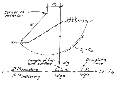
The weight of the soil is driving the soil downward, and this is resisted by the shear resistance along the failure surface (the dashed line.) That resistance is affected by a number of factors, including effective stress along the failure surface, friction of the particles, and cohesion of the soil. The whole mass rotates about the center of rotation, which has to be determined during analysis.

The most common method used–and the one SLOPE uses–is the method of slices. In that method the soil mass is divided into vertical slices, each of which has a mass, some kind of resistance along the failure surface, and (for most of the methods used) how the slices interact with each other.

The theory is described in both Soil Mechanics and the Soils and Foundations Reference Manual. The computations can be laborious, but the really tricky part is determining the location of the center of rotation and the radius R of the failure surface. SLOPE takes care of all of that but it is essential for you to understand how it does that, as its determination of all of these factors is not automatic.

Dealing With Different Expressions of Slope

One common problem with slope stability situations is how the geometry of the slope is defined. There is more than one way of doing it, and the method used in the problem is different than the one used in SLOPE.

The problem states that the slope is 35′ high (the vertical length of the slope) with a grade of 1.5H/1V. This means that, for every foot or meter of height, there are 1.5 feet or meters of horizontal length. In this case the horizontal length is (35)(1.5)/(1) = 52.5′. Alternatively we can compute the angle of slope as arctan(1/1.5) = 33.7 degrees, in which case the length is 35/tan(33.7) = 52.5′

Inputting the Data

SLOPE requires the data to be put in SI units. We will do the conversions as we proceed. The data input is as follows:

Length of slope (m) = 52.5′ = 16 m
Height of slope (m) = 35′ = 10.7 m
Water level left side (m) = 0 (from problem statement, zero is at the toe of the slope)
Water level right side (m) = 0 (again from problem statement)
Unit weight of water (kN/m³) = 10 (reasonable approximation)
Dry unit weight of embankment* (kN/m³) = 120 pcf = 18.9 kN/m³
Saturated unit weight of embankment (kN/m³) = 18.9 (in absence of better data, use the same)
Cohesion soil in embankment (kN/m²) = 500 pcf = 23.9 kN/m²
Friction angle in embankment (degrees) = 20 (from problem statement)
Neutral stress coefficient subsoil** = 1.00
Dry unit weight subsoil* (kN/m³) = 120 pcf = 18.9 kN/m³
Saturated unit weight subsoil (kN/m³) = 18.9 (in absence of better data, use the same)
Cohesion soil subsoil (kN/m²) = 1,000 pcf = 47.9 kN/m²
Friction angle subsoil (degrees) = 0 (from problem statement)
Neutral stress coefficient embankment** = 0.66
Lower left corner window*** – x(m)
Lower left corner window*** – y(m)
Upper right corner window*** – x(m)
Upper right corner window*** – y(m)
Deepest point of slip circles – y(m) = -25′ = -7.6 m (this is negative as it is below the toe of the slope)

Notes:
* The embankment is above the toe. The subsoil is below it.
** The neutral stress coefficient is more commonly referred to in American practice as the at-rest earth pressure coefficients. For normally consolidated soils, it equals to $1 - \sin(\phi)$ , and the results are shown in the input list. The entry points for both are out of order, so be careful.
*** This will be explained below.

Choosing the Window Points and the Method of Analyzing the Slices

If we put all of this data into SLOPE, we get the following result:

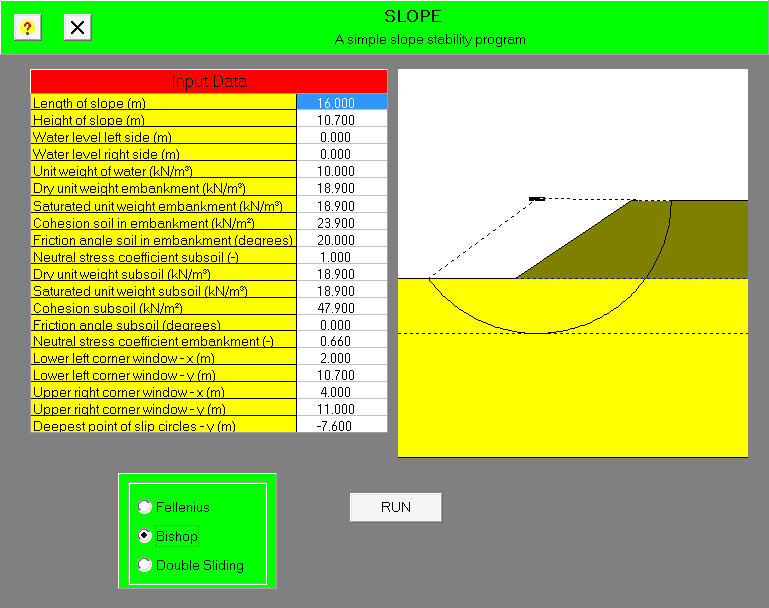
Before we get some results, we have to make two decisions: what slice analysis method to use and the extent of the window.

Soil Mechanics gives an explanation of Fellenius and Bishop’s methods. SLOPE divides the region in the slip circle into the horizontal slices; the difference between these two methods is that Fellenius’ method does not consider friction between the slices while Bishop’s does. Fellenius’ method does not require an iterative solution and is the most conservative; however, given that the computational effort is done by the program, we will use Bishop’s method, which is in common use.

As far as the “window” is concerned, SLOPE, in common with many slope stability programs, uses a grid optimization method to find the location of the rotational centre. This means that a set of points in a regular grid are each analyzed (along with appropriate slip circles) to get the factor of safety (see sketch above) and after analyzing all of these points picks the one with the lowest factor of safety. It’s easy to see that, using the original grid, not much in the way of useful information can be found as the selection of grid points is too small. For a grid point to be valid, it has to be in the interior of the window, not at the edge, because if it’s at the edge it’s possible that the point will be outside of the window.

The window limits are set using a coordinate system with the origin at the toe of the slope. Generally the slip circle centre will be above and to the left of the upper corner of the slope. Values for y should not be less than the slope height and values for x should be greater than zero and less than the length of the slope.

Getting an acceptable result is an iterative process. Let us assume the following for the window boundaries:

Lower left corner window*** – x(m) = 2 m
Lower left corner window*** – y(m) – 10.7 m
Upper right corner window*** – x(m) – 14 m
Upper right corner window*** – y(m) – 15 m

If we apply these and then Bishop’s method for the analysis, we get the following result:

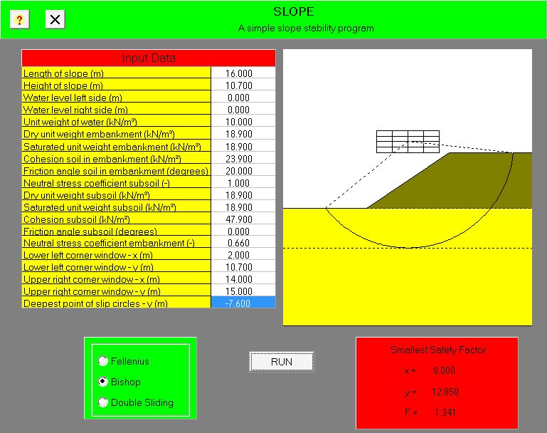
We can see the slip circle centre is in the interior of the grid. If we desire we can shrink the window to get a finer grid and a more precise result.

Sometimes assuming the slip circle going to its lowest point does not result in the lowest factor of safety. To simulate something close to a toe circle, let us set the deepest point at the bottom of the embankment; the result we obtain is as follows:

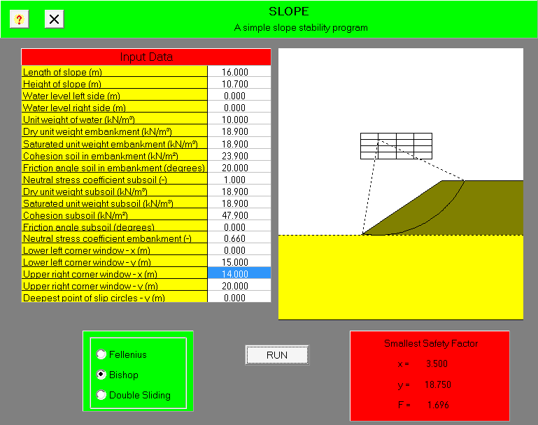
In this case (with some adjustments to the window) the factor of safety is still higher for our original case.

Reporting the Results

SLOPE is not installed, and as a result does not print out its results. The only way to save the results from the program is to get them off of the screen. This is fairly straightforward: use a grab or screenshot program, which was done with the images in this post. Unfortunately many of my students, for whatever reason, insisted on using their phones to take shots of the literal screen, which generally look awful. This was the technology I used forty years ago when presenting this program; we’ve come a long way since.

Conclusion

SLOPE is a fairly simple program to use. It lacks many of the automation and stratigraphy defining features other slope stability software packages have, and is not suited for use in practice. For academic use, however, it is good, and gets students past one of the most tedious features of geotechnical computation.

Geotechnical Engineering, Soil Mechanics

Why Only Rankine?

Posted on 17 August 2026 by Don Warrington

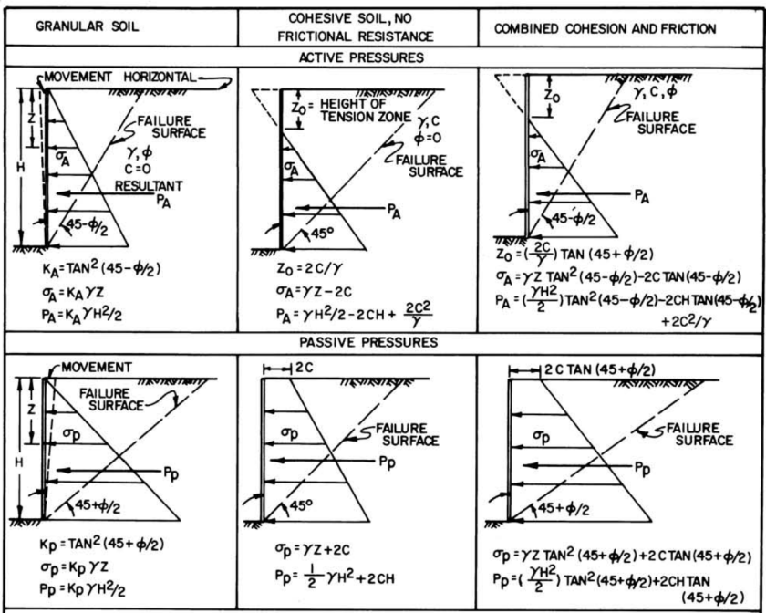
With release of Soils in Construction, Seventh Edition, we now turn to discuss some of the special topics surrounding this book. One of them is the earth pressure theory we adopted: Rankine earth pressures, level backfill, with provision (when necessary) for cohesive soils. For a textbook this seems awfully restrictive, but there are justifications for this policy.

Rankine earth pressure theory is the most elementary of the earth pressure theories. It is customary, however, in introductory geotechnical courses such as Soil Mechanics and Foundation Design and Analysis, to present all three failure criteria (Rankine, Coulomb and Log-Spiral.) For many years I did so in the first course and went back to expand on that in the second; it was the only topic I formally reviewed from one semester to the next. In spite of that, my students found the topic confusing, never sure which theory applied even when I made it clear (or so I thought.) What I ended up doing was teaching strictly Rankine theory in Soil Mechanics and the others in Foundation Design and Analysis.

Rankine is also characterised as the most conservative of the earth pressure theories. In his response to a paper by Terzaghi (reviewed for other reasons in my post An Industry Gets Restless: Terzaghi’s 1929 Paper on Dynamic Formulae and the Response) Lazarus White made the following observation:

In the Nineties, when the writer was an undergraduate student, he was thoroughly imbued with the classical methods of computing earth pressures, bearing values of soil, distribution of pressures, and pile-driving formula commonly taught–Rankine, Baker, Cain and Wellington–and, after his graduation, he set about to apply them…Later, during subway construction, he observed that contractors completely and successfully ignored Rankine and Cain in timbering work, and “got away with it” in so many instances that by no scientific philosophy could their theories be justified.

Of the four methods he mentions, only Rankine is still taught as a “currently” used method, although it too is being displaced by methods such as FEA. So how can the decision to teach only Rankine in Soils in Construction be justified? It is done as follows:

It’s good that White’s result was “got away with it” and not a collapsed wall; retaining wall failures tend to be catastrophic. It kept his work out of trouble until better methods could be employed.
It was the policy of previous editions of the book, although some attempt has been made to use Rankine in conjunction with Mohr-Coulomb for a theoretically consistent presentation.
Soils in Construction is primarily aimed at giving contractors a better understanding of geotechnical issues, not as a design guide. It can be taught in a more geotechnical engineering way but its first task is contractor education.
Some introductory geotechnical courses only teach Rankine theory with level backfill, such as Tsytovich, which came as something of a shock to me. Either proficiency in more advanced theories were left to experience or later courses for specialists.
As noted and in common with NAVFAC DM 7.2, only level backfill is considered, as discussed in my post NAVFAC DM 7.2: Analysis of Walls and Retaining Structures, Part I: Will the Real Rankine Theory Please Stand Up?. Rankine theory can be extended to sloping backfills but again we did not feel this was necessary for a book such as Soils in Construction.
Rankine theory with level backfill is the only theory necessary to take the FE exam; preparation for this was one of the objectives of the “extended” material in the book.

Uncategorized

NAVFAC DM 7.2: Earthwork, Hydraulic and Underwater

Posted on 17 April 2025 by Don Warrington

The whole topic of earthwork and compaction is one whose coverage is inconsistent, to say the least, in basic geotechnical publications. Some do a very good job, others ignore it altogether. NAVFAC DM 7.2 has done a very thorough job on the subject, covering topics which are scarce in other places. Compaction is the oldest earth improvement technique we have and is still the most commonly used on construction sites around the world.

There are many topics which are explored in this chapter; I will only mention a few of them. It’s hard to distill all of the information in the book; you’ll just have to get it and find out for yourself. Some of them (such as compaction equipment types and sample fill specifications) are carried over and expanded from the previous document; others are new.

Line of Optimums Method

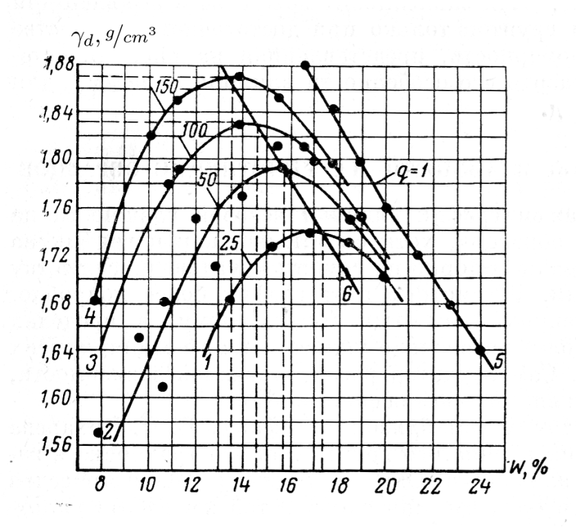
When I was first brought on board to Soils in Construction, I learned about this, which I discuss in this post (illustration of the method is at the right.) There were few references on the subject to be found, which made Soils in Construction somewhat unique. (I need to say kudos to my co-author, Lee Schroeder, especially for the part of the book on compaction.) We actually got thumbs up during the review process for including it. This edition of NAVFAC DM 7.2 has fixed that lacuna with a section on the subject. I don’t see how one can actually specify a compaction method without it, especially if experience is lacking and/or the soils are variable on a site. They have included information on the effects of “dry of optimum” (left of line 6 on the chart above) and “wet of optimum (right of line 6) as well. All in all, a very nice treatment on the subject.

Making the Cut with Borrow and Fill Calculations

Another topic covered in Soils in Construction is that of borrow and fill calculations. Some soil mechanics books cover this, some don’t. It’s covered in detail in NAVFAC DM 7.2. It will definitely help you to “make the cut” when excavating, transporting, placing and compacting fill materials.

Hydraulic Fills

Many geotechical references treat hydraulic fills as a thing of the past after some early disasters involving them. Evidently not; there is a whole chapter on the subject, both for understanding dams built in this way and for underwater fills, when hydraulic fills are virtually unavoidable.

Civil Engineering, Geotechnical Engineering

NAVFAC DM 7.2: Geotechnical Design in Problem Soils and Specialty Construction Methods

Posted on 4 April 2025 by Don Warrington

This week we’ll look at the first chapter of the book. The whole business of “problem soils” is not straightforward because it’s a matter of degree. Given the nature of soils vs. other engineering materials, all soils are problem soils; it’s just that some soils pose a greater problem to those of us who choose to build on, under or next to them than others, greatly so in some cases.

Most of the problem soils identified in the chapter are clays: loess, expansive soils, residual silts and clays, etc. Organic soils are included in this list, although the best way to deal with most of these is to avoid them altogether. Most of the descriptions of these soils is qualitative rather than quantitative, and that’s the weakness of the whole discussion. While general awareness of these soils and the challenges they create is useful, some quantitative description would have been useful.

An example of this is the determination of the growth of expansive soils with changing water content. Many of the studies of the volume change in these soils produce results that are either too specific or too difficult to readily implement either in an academic setting (where qualitative discussions of these soils abound) or in practice. Some of this is addressed in DM 7.1, but a more thorough approach would have been appreciated. I tackled this issue by presenting van der Merwe’s method in a more detailed fashion than usual; some more of this here would have been helpful.

The last part of the chapter deals with specialty construction methods in a page diagram reminiscent of the old driven pile diagrams from the previous edition. These are helpful because many proprietary methods don’t get the coverage in undergraduate texts that would be useful in the field. Fortunately in these cases specific references to more detailed descriptions–including design information–are given. The documents referred to are available on this site.

And a word of thanks…

I want to thank all of you who ordered the new DM 7.2 after its introduction last month. And that was quite a few of you: this has been the most successful publication launch of any book I have offered since I started doing this in 2006. Thank you so much for your support of our publications; it means a great deal for the continuation of this site.

And then there was another surprise last week in the video launching of the book from the Geo-Institute:

Notice the book cover on the splash screen? I had no idea they would do that. The first volume noted that it had been on the bookshelves of engineers for many years, and at this point the only way to acquire these books in print (AFAIK) is here.

Academic Issues, Geotechnical Engineering

Explaining the Relationship Between the Coefficient and the Angle of Friction

Posted on 28 October 2024 by Don Warrington

One of the things that gets covered (if not very thoroughly) in Soil Mechanics is how friction is developed in soils. An analogy is made with the classic “block on a surface” problem we see in Statics, but the tie-in isn’t as strong as one would like.

The fact is that, for purely cohesionless soils, the friction between the particles and the friction between the surface and the block is basically the same Coulombic friction. As is usually the case in soil mechanics, how that actually plays out in soil properties has many complexities, but then again surface friction isn’t a simple or straightforward property in and of itself.

Another part of the problem is that, in Statics, friction isn’t taught with geotechnical considerations in mind, especially these days. This is a pity, not only for those of us in the geotechnical community but for those who work with granular materials on a production or use basis.

This is a brief treatment of the subject, basing the development of the topic from that in Movnin and Izrayelit (1970), which comes closer to relating the two quantities we see to define friction: the friction angle and the friction coefficient.

The Basics of the Friction Coefficient and Angle

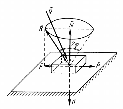
Surface friction comes from the rubbing of two surfaces together, as shown at the right. We see the three forces with which the two surfaces interact: the normal force N, the resulting friction force F and the resultant of the two R. We also see that the addition of lubricant is important in that it separates the two surfaces and reduces the effect of the asperities on each other, something that contractor and engineer alike frequently overlook in both the maintenance and performance evaluation of the equipment.

The normal and frictional forces resisting the relative motion of the two surfaces is related by the equation

F = fN (1)

With granular materials, the main difference is that the surfaces of the particles aren’t straight at all but they do rub up against each other, the asperities on the particle surface contributing to the mutual resistance of the particles. Although water acts to a limited extent as a lubricant, its largest effect is the buoyant effect on the intergranular (effective) stress, as shown below.

Returning to the first diagram, without any mutual pressure of the surfaces (the normal force N) there is no friction force F tangential to the surface. Again in soil mechanics purely cohesionless (granular) soils have no frictional strength unless weight or other pressure is applied to them.

Diagram of forces on a body on a plane surface with friction, from Movnin and Izraelyt (1970)

Now let us consider the diagram at the right. The normal force N exerted by the surface on the block (caused by the force exerted on the block Q) and the frictional force F (caused by the force P which attempts to move the block) add vectorially to a resultant R, which in turn has an angle with the normal force N. The geometry of the forces and Equation (1) relate the angle to the friction factor as

f = F/N = tan (φ) (2)

Cone of Friction

Although F and N are related through both Equations (1) and (2), in reality F cannot exist without some tangential force pushing the block. This is the force P which is attempting to push the block along the plane. As P increases F increases until we get to a point where we have impending motion, beyond which the block moves and begins to accelerate. The value of f or φ when impending motion turns into actual motion is when we reach the ultimate value of f or φ, which we will designate as f₀ or φ₀.

These form a “cone of friction.” This cone of friction can be seen in the diagram at the left. As long as F < f₀ N (or F < tan (φ₀) N) and the resultant Q of N and F is within the cone, the block is motionless. Beyond that point it moves, and the coefficient of friction in motion can be different (usually smaller) than the coefficient of friction at the point of impending motion.

It is here that we can relate the friction factor f and the angle of friction φ can be related to each other and to concepts familiar to geotechnical people. When we construct the Mohr-Coulomb diagram, we define a failure envelope of legal stress states (within the envelope) and illegal stress states (outside the envelope.) We can see all of these with the failure function below. When the failure function is negative (1), we are within the envelope and failure does not take place. When the failure function is zero (2), we have impending failure. When the failure function is positive (3), we have failure and an illegal stress state.

Three-dimensional envelopes are certainly common in geotechnics, especially in finite elements. An example of this is shown below.

Determining the Friction Factor or Angle

Determining the angle of friction, from Movnin and Izraelit (1970)

To determine the friction angle, one simple way is to start with a block and a level surface and then raise the angle of the surface until the block moves. Such an apparatus is shown at the left.

As the angle α increases the direction of the weight G relative to the surface changes in can be divided into two parts: the normal force G₂ and the tangential force G₁. The latter will move the block down but it is resisted by the friction force F, which will resist until G₁ > F₀, at which point the block will start to move down the slope at a constant acceleration. By noting the angle at which this takes place, both f₀ or φ₀ = α₀ can be determined. The math for this is similar to the level surface and block.

The geotechnical counterpart to this is the angle of repose. Suppose we allow a small stream of sand to drop on a surface. Over time the sand will build up into a conical pile with the surface at an angle to the flat surface the sand is streamed onto. This angle is referred to as the angle of repose. In theory the angle of repose is equal to the friction angle of the soil, although with the usual complexities of geotechnics this isn’t always the case. There are clean sands with which we can use the angle of repose to estimate the internal friction angle of the soil. When I was teaching at UTC, some of the students were working on the ASCE MSE Wall project and needed a friction value for the sand being used in the box. While they were looking at direct shear or triaxial testing, I suggested using the angle of repose to get a “ballpark” value. They did this and it was helpful.

Some Comments

The use of the angle of friction has fallen out of favour in engineering education, which is one reason why it is difficult to relate friction as taught in Statics to friction as used in geotechnical engineering. That wasn’t always the case; one example from the early twentieth century is Tapered Keys and Their Use In Vulcan Hammers.
Hopefully this treatment of the subject will be useful to students to help them relate the concept of friction in statics to that in geotechnical engineering.