vulcanhammer.net

A First Look at Estimating Beta Factors for Determining Pile Shaft Capacity of Driven Piles

Posted on 4 October 201726 May 2025 by Don Warrington

In the last posting about STADYN, we put forth considerations for interface elements between the pile shaft and the soil. Before we formally incorporate these into the model (or whether we will incorporate them or not) some consideration of how the interface actually works. We will start those considerations by looking at methods by which the static capacity of driven piles is computed, and specifically the so-called “beta” methods which are used for cohesionless and sometimes cohesive soils.

Beta methods assume that the shaft resistance of the pile is a function of the effective stress of the soil along the pile shaft. They assume that the horizontal stress that results from the vertical stress acts perpendicular to the surface of the pile. The pile surface thus acts like a block on a surface with some kind of Coulombic friction acting against the downward settlement of the pile. The beta coefficient is the ratio between the vertical effective stress and the horizontal friction on the pile, or

$f_s = \beta \sigma'_o$

$\beta$ is in turn broken down into two components: the lateral earth pressure coefficient, which is the ratio between the horizontal and vertical stresses,

$K = \frac {\sigma_h}{\sigma'_o}$

and the coefficient of friction, or

$\mu = tan \phi$

We put these together to yield

$\beta = K tan \phi$

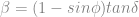
At this point let’s make two assumptions. The first is that the lateral earth pressure coefficient is in fact the at-rest lateral earth pressure coefficient. (For some discussion of this, you can view this slide presentation.) The second is that the friction angle between the pile and the soil is in fact the same as the soil’s internal friction angle. If we use Jaky’s formula for the at-rest condition, these assumptions yield

$\beta = \left (1-\sin(\phi)\right )\tan\phi$

The various components of this equation are plotted below.

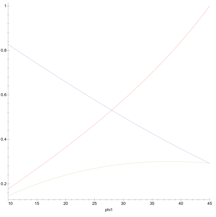
The three lines are as follows:

$K_o = 1 - sin \phi$ is in red.
$tan \phi$ is in blue.
$\beta$ is in green.

It’s interesting to note that, as $K_o$ increases, $tan \phi$ decreases, and so $\beta$ is within a surprisingly narrow range of values. This plot is similar to one shown in Burland (1973), which we will discuss later.

If this were the case in practice, estimating $\beta$ would be a straightforward proposition. We’ll take two examples to show that this is not the case.

Let’s start with the Dennis and Olson Method for cohesionless soils, which is described here. To arrive at $\beta$ they do the following:

They add a depth factor, which we will not consider. Depth factors and critical lengths are common in static methods, but they are not well documented in the field.
They assume $K_o = 0.8$ if their values for friction angle are used.
They vary the friction angle from 15-35 degrees depending upon the type of soil.

Leaving out the depth factor, for this method $\beta$ ranges from 0.21 to 0.56. This is a considerably wider variation than is indicated above. Since the depth factor is frequently greater than unity, this range is even larger.

An easier way to see this is to consider the method of Fellenius. His values for $\beta$ are as follows:

0.15-0.35 for clay
0.25-0.50 for silt
0.30-0.90 for sand
0.35-0.80 for gravel

Again the range of values is greater than the figure above would indicate. Why is this?

Although it’s tempting to use a straight empirical approach, let’s back up and consider the structure of the basic equation about and the assumptions behind it. There are several ways we can alter these equations in an attempt to match field conditions better by considering these assumptions and seeing what changes might be made.

The Two Friction Angles Aren’t the Same

The first one is suggested by the notation in Dennis and Olson: the internal friction angle of the soil and that of the soil-pile interface are not the same. Retaining wall theory (when it considers friction) routinely makes this assumption; in fact, the ratio $\frac {\delta}{\phi}$ routinely appears in calculations. Let us rewrite the equation for $\beta$ as

$\beta = (1 - sin \phi) tan \delta$

and be defining the ratio

$m = \frac {\delta}{\phi}$

we have

$\beta = (1 - sin \phi) tan (m \phi)$

If we plot this in a three-dimensional way, we get the following result.

$\beta$ is the vertical axis; m is varied from 0.25 to 1.75. The results show that, for a given $\phi$ , if we increase m we will increase $\beta$ , and this increase is much more pronounced at higher values of $\phi$ .

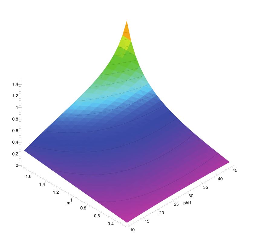
Although it’s certainly possible to have very high values of $\delta = m \phi$ , as a practical matter in most cases m < 1. Nordlund’s Method, for example indicates that m > 1 only with tapered piles, where a tapered pile face induces some compression in the soil in addition to shear. In any case is m < 1 this will tend to depress values of $\beta$ . We should also note that using a ratio m does not mean that it will be a constant for any given soil. This is especially true if $\phi = 0$ , where a multiplier is meaningless and we should have recourse to an additive term as well.

Jaky’s Equation Doesn’t Apply, or At-Rest Earth Pressure Conditions Are Not Present

Another assumption that can be challenged is that Jaky’s Equation doesn’t apply, or we don’t have at-rest earth pressure conditions. Although Jaky’s Equation has done well, it is certainly not the last word on the subject, especially for overconsolidated soils (which we will discuss below.) To try to “cover our bases” on this, let’s consider a range of lateral earth pressure coefficients by assuming that Jaky’s Equation is valid for the at-rest condition and that we need to somehow vary between some kind of active state and passive state. The simplest way to do this is to assume Rankine’s conditions with level backfill, which just happens to be identical to Mohr-Coulomb relationships between confining and driving stresses. (OK, it’s not all luck here…) Thus,

$K_a = \frac {1-sin\phi}{1+sin\phi}$

and

$K_p = \frac {1+sin\phi}{1-sin\phi}$

Let us also define an active-passive factor called actpas, where actpas = -1 for the active state, 0 for the at-rest state and 1 for the passive state. We then plot this equation

$\beta = K(\phi,actpas) tan \phi$

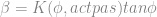
below. Since we only have K values for three values of actpas, we’ll use a little Lagrangian interpolation in an attempt to achieve a smooth transition between the states.

We note from this the following:

The dip in $\beta$ for the high values of $\phi$ and -1 < actpas < 0 (states tending towards the active) may be more a function of the interpolation than the physics. OTOH, if we look at NAVFAC DM 7.02, Chapter 3, Figure 1, we see a dip between the at-rest and active states for dense sands, which is what we would expect at higher values of $\phi$ .
Values of $\beta$ for the active case show little variation. Given that driven piles are subject to cavity expansion during installation, one would expect some passivity in earth pressures. Drilled shafts are another story; however, if we look, for example, at O’Neill and Reese, values for $\beta$ can certainly range higher than one sees with the active states above. Bored piles, however, are beyond the scope of this discussion.
For low values of $\phi$ , there is little variation between the three states.
If we compare these values with, say, those of Fellenius or Dennis and Olson, we cannot say that the fully passive state applies for most reasonable values of $\phi$ , undrained or drained. (Values in Nordlund, however, indicate higher values of K for larger displacements, approaching full passivity for large displacement piles. Another look at this issue is here.)

Conclusion

If we compare the results we obtain above with empirical methods for determining $\beta$ , we see that none of the variations shown above really allows us to match the theory we’ve presented with the empirical methods we’ve described (and others as well.) As a general rule, $\delta < \phi$ or $m < 1$ , so it’s safe to conclude that our assumption that the $K$ can be determined using Jaky’s Equation only results in values of $\beta$ that are too low.

It’s tempting to simply fall back on an empirical value for $\beta$ , but for finite element analysis a more refined approach seems appropriate. In subsequent posts we’ll look at such an approach, along with the issue of applying $\beta$ methods to cohesive soils as well as cohesionless ones.

References

In addition to those in the original study, the following reference is mentioned here:

Burland, J.B. (1973) “Shaft friction of piles in clay – A simple fundamental approach.” Ground Engineering 6(3):30-42, January.

Uncategorized

Some Things I Would Say if Giving the E.A.L. Smith Award Lecture for the Pile Driving Contractors Association

Posted on 21 September 201726 May 2025 by Don Warrington

I found it intriguing that the Pile Driving Contractors Association has instituted the E.A.L. Smith Award with lecture following. It looks like I’ve already made a contribution to the effort: the graphic they used for the LinkedIn announcement probably comes from my piece on E.A.L. Smith and his contribution.

I don’t anticipate actually doing this, but that’s the result of some choices I’ve made along the way.

To begin with, I allowed my technical membership in PDCA to lapse many years ago, although the organisation I work for certainly is a member. As the musicians say, you can’t sing the blues if you don’t pay your dues, and that’s as true in deep foundations as it is in jazz music.

Beyond that, most people who have been in the driven pile industry for a while know that Vulcan Iron Works passed from the Warrington family in 1996, and that things really didn’t get better for some time thereafter. My years in the equipment business convinced me that equipment people could not remain uninvolved in the whole business of pile dynamics, which led me to start this site twenty years ago. Unfortunately that involvement was not accompanied by a sponsoring organisation or budget, so I had to use the emerging internet to do what I felt needed to be done: furnish information on pile dynamics and driven piles, and ultimately geotechnical and marine engineering in general, without paywall or restriction. That effort has been successful; the award for it is in geotechnical engineers who can get their work done in a better way, students who can learn about this part of the profession, and those in countries which lack the resources to purchase materials. If I’ve helped them, I’ve succeeded, and that’s award enough.

In any case part of that effort was my piece on E.A.L. Smith and his development of the wave equation program, and I think my piece has been just about the only one on the subject for a long time. In looking back at the piece and the whole effort behind it, I’d like to make some observations that hopefully with shed some light on Smith’s effort.

The first is that Smith was Raymond’s Chief Mechanical Engineer. Raymond was an organisation that defined vertical integration: they not only drove the piles, but made or modified the equipment that did the work. Smith worked during an era when geotechnical engineering was coming into maturity as a science; Terzaghi and Peck’s Soil Mechanics in Engineering Practice was published in 1947. Nevertheless it took a mechanical engineer to crack the forward problem in pile dynamics. That’s because civil engineers in general and geotechnical engineers in particular don’t really like or understand things that move, but moving things (like pile driving equipment) are the centrepiece of a mechanical engineer’s work. That simple fact invited the interdisciplinary approach to the problem that Smith took, but it also has made pile dynamics a “black box” to many of the civil engineers who work with the problem, and that in turn has guided the way the solution of the problem has been implemented.

The second is that the physics of Smith’s wave equation program is a classically mechanical engineer’s solution to a problem. Spring-dashpot-mass systems are the core building blocks of any vibrating system; Smith basically took this, made the springs elasto-plastic, and strung them together into the system he developed. It is a tribute to Smith’s ability to see the big picture of the system to relate the parameters of the system to the soil he was driving into, and not permit himself to get lost in the soil mechanics of his geotechnical peers.

The third is that Smith developed his numerical method at a time when numerical simulation of physical systems was itself in its infancy. He had the feedback of the likes of W.E. Milne and the collaboration of crosstown IBM’s computers and expertise in the development. It’s also worth noting that civil engineering, although it has pushed forward finite element modeling with people such as T.J.R. Hughes and D. Vaughn Griffiths, is still content with using “classical” methods for many of its designs, especially in the transportation field. The singularity of Smith’s achievement needs to be seen in the context of both the situation at the time and afterwards.

The fourth is that Smith’s wave equation program was the result of an extended effort that lasted at least a decade and probably more. That was facilitated by Raymond itself, a large organisation with considerable resources and the ability to test the model with its own work. It was done at a time when U.S. corporations were more inclined to engage in long-term research projects and to share those results. The government’s involvement only entered in the wake of Smith’s seminal ASCE paper, and that too was an extended effort.

So Smith’s effort is certainly worthy of celebration and commemoration, and to learn some lessons from it. Smith’s basic model of the pile has endured to this day, finding application in both forward and inverse solutions of the wave equation for piles. But is Smith’s model the last word on the subject? Probably the best answer came from Smith himself. In his ASCE paper he noted the following, in his discussion of soil mechanics:

When future investigators develop new facts, the mathematical method explained herein can be modified readily to take account of them…

It’s unreasonable to expect that Smith’s model cannot be improved on beyond tweaking the parameters. And there are fundamental problems: Smith, wise to initially bypass much conventional soil mechanics, developed a model where the relationship between the parameters he used and the properties of the soil he was driving into is not clear. Solving that problem might, for example, reduce the importance of the sensitivity issue of soil damping on the results of the wave equation. Efforts have been made to solve the model-soil properties issues but they are neither as widely perfected or implemented as one would like.

That’s a special problem when he consider the inverse implementation of the wave equation for piling. Use of Smith’s model brings with it uniqueness issues (and there are enough of those with problems involving plasticity like this one) that need to be addressed.

Numerical methods and computer power have both vastly improved since Smith’s day. So is it possible to see another paradigm shift in the way we perform forward and inverse pile dynamics? The answer is “yes,” but there are two main obstacles to seeing that dream become a reality.

The first is the nature of our research system. As noted above, Smith’s achievement was done in a large organisation with considerable resources and the means to make them a reality. It was also a long-term effort. Today the piecemeal nature of our research grant system and the organisational disconnect among between universities, contractors and owners incentivises tweaking existing technology and techniques rather than taking bolder, riskier steps with the possible consequence of a dead-end result and a disappointed grant source.

The second is the nature of our standard, code and legal system. Getting the wave equation accepted in the transportation building community, for example, was an extended process that took longer than developing the program in the first place. Geotechnical engineering is a traditionally conservative branch of the profession. Its conservatism is buttressed by our code and standard system (which is also slow-moving) and the punishment meted out by our legal system when things go wrong, even when the mistake was well-intentioned. Getting a replacement will doubtless be a similar extended process. And of course we should consider having been “written into the specs.” Vulcan was certainly the beneficiary of that phenomenon, although the process was driven more by the ubiquity of the product than an effort by the company. That last point is certainly not the case here; general acceptance would have never taken place had it been so.

However, we need to face the reality that, sooner or later, the ball will move down the field and newer techniques will be developed. The question in front of us is whether it will be done on these shores, as was the case with Smith, or somewhere else. As I like to say, it’s our move: we need to make it.

Uncategorized

STADYN Wave Equation Program 4: Eta Limiting, and More on Norm Matching

Posted on 24 August 201726 May 2025 by Don Warrington

In our last post we broached the subject of different norm matching methods for the actual and computed velocity-time histories at the pile top. In this post we will go into $\eta$ limiting, while at the same time running both norms to get a better feel for the differences in the results.

Before we begin, one clarification is in order: CAPWAP’s Match Quality and the use of the 1-norm in STADYN are similar in mathematical concept but different in execution. That’s because the Match Quality weights different part of the force-time history (in their case) differently, whereas STADYN goes for a simple minimum sum difference.

One characteristic of the inverse case both in the original study and in the modifications shown in the last post are very large absolute values of $\eta$ . These are products of the search routine, but they are not very realistic in terms of characterising the soil around the pile. To illustrate, we bring back up one of the results from the last post, showing the optimisation track using the 2-norm and phi-based Poisson’s Ratio (which will now be the program standard):

Note that the #8 track ( $\eta$ for the lowest shaft layer) has a value approaching -30; this is obviously very unrealistic.

In principle, as with $\xi$ , the absolute value of $\eta$ should not exceed unity; however, unlike $\xi$ there is no formal reason why this should be the case. But how much should we vary $\eta$ ? To answer this question, and to continue our investigation of the norm issue, we will examine a matrix of cases as follows:

$\eta$ will be run for values of 1, 2, 3 and unlimited (the last has already been done.)
Each of these will be run for both the 1-norm and 2-norm matching.

A summary of the results are shown below

Changed Parameter	Difference		Static Load, kN		Average Shaft $\xi$		Toe $\xi$		Toe $\eta$
Norm	1	2	1	2	1	2	1	2	1	2
\| $\eta$ \| < 1	0.3364	0.003690	811	1490	-0.364	-0.149	-0.62	-0.311	-0.175	0.611
\| $\eta$ \| < 2	0.2381	0.002626	278	223	-0.091	-0.06	-0.588	-0.316	-0.781	-0.0385
\| $\eta$ \| < 3	0.1806	0.001707	172	207	0.324	0.42	-.832	0.823	-1.01	1.45
Unrestricted $\eta$	0.1344	0.001456	300	218	-0.329	-0.183	-0.491	0.804	8.19	1.52
$\nu = f(\xi,\eta)$	0.1484	0.001495	278	187	-0.383	-0.53	0.792	0.366	3.116	1.814

To see how this actually looks, consider the runs where | $\eta$ | < 3. We will use the 2-norm results.

Velocity-Time Output — Impedance*Velocity Comparison, 2-norm, eta limiting = 3.

Optimization Track — Optimisation Track, 2-norm, eta limiting = 3

The results indicate the following:

The average shaft values of $\xi$ tend to be negative. This is contrary to the cohesive nature of the soils. The interface issue needs to be revisited.
The toe values do not exhibit a consistent pattern. This is probably due to the fact that they are compensating for changes in values along the shaft.
As values of | $\eta$ | are allowed to increase, with the 2-norm the result of the simulated static load test become fairly consistent. This is not the case with the 1-norm. Although limiting | $\eta$ | to unity is too restrictive, it is possible to achieve consistent results without removing all limits on $\eta$ .
The velocity (actually impedance*velocity) history matching is similar to what we have seen before with the unlimited eta case.
The optimisation track starts by exploring the limits of $\eta$ , but then “pulls back” to values away from the limits. This indicates that, while limiting values “within the box,” i.e., the absolute values of $\eta$ < 1, is too restrictive, reasonable results can be obtained with some $\eta$ limiting.

Based on these results, $\eta$ limiting will be incorporated into the program. The next topic to be considered are changes in the soil properties along the surface of the pile, as was discussed in the last post.

STADYN

STADYN Wave Equation Program 3: Match Quality vs. Least Squares Analysis

Posted on 5 July 201726 May 2025 by Don Warrington

Having broached the subject of Poisson’s Ratio and how it is computed for forward methods, we can turn to how it affects inverse methods. However, at the same we need to consider an issue that is vital to understanding either this method or methods such as CAPWAP: how the actual pile head signal is matched with the signal the model proposes. There is more than one method of doing this, and the method currently used by CAPWAP is different than what is widely used in many engineering applications. Is this difference justified? First, we need to consider just what we are talking about here, and to do that we need a brief explanation of vector norms.

Vector Norms

A vector is simply a column (or row) of numbers. We want to compare vectors in a convenient way. To do this we must aggregate the entries in the vector into a scalar number, and we use what we call norms to accomplish this. In theory there are an infinite number of ways to do this: according to this reference, there are three types of norms in most common use, they are as follows:

stadyn3norms — Left: the 1-norm. Center: the 2-norm, or Euclidean norm. Right: the infinity-norm.

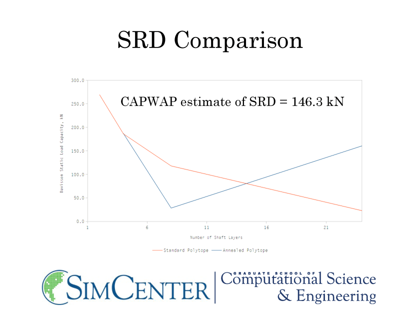
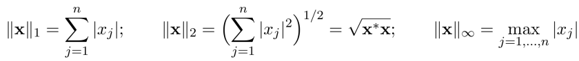
So how do use norms in signal matching? We reduce the force-time (or in our case the velocity-time) history at the pile top after impact into a series of data points, and then for each point of time of each data point we compute the results our proposed model gives us and subtract it from the actual result. In the equation above each data point is a value $x_j$ . When we have all the differences in hand, we take them and compute a vector of differences, and then in turn take the norm of those differences. We do this successively by changing parameters until we get a norm value which is the minimum we can reach. For the STADYN program, we use the $\xi - \eta$ values as parameters and iterate using a polytope method (standard or annealed, for our test case the latter.)

For our purposes the infinity norm can be eliminated up front: in addition to having uniqueness issues (see Santamarina and Fratta (1998), we have enough of those already) it only concerns itself with the single largest difference between the two data sets. Given the complexities of the signal, this is probably not a good norm to use.

That leaves us with the 1-norm and 2-norm. To keep things from getting too abstract we should identify these differently, as follows:

1-norm = “Match Quality” for CAPWAP (see Rausche et. al. (2010))
2-norm = Least Squares or Euclidean norm (think about the hypotenuse of a triangle.) This relates to many methods in statistics and linear algebra, and has a long history in signal matching (Manley (1944).) This is what was used in the original study.

One thing that should be noted is that the norm we actually use is modified from the above formulae by division of the number of data points. This is to prevent mishap in the event the time step (and thus the number of data points) changes. However, for the Mondello and Killingsworth (2014) pile, the wall thickness of the steel section drove the time step, which did not change with soil changes; thus, this division is immaterial as long as it is done every time, which it was.

Application to Test Case

As noted earlier, we will use the four-layer case using the annealed polytope method of matching. Let us start at the end, so to speak, by showing the static load test data that the program runs with the final configuration:

Davisson Load, kN	Original $\nu$	$\phi$ -based $\nu$	% Change
1-norm	278	300	7.91%
2-norm	187.1	218	16.52%
% Change	48.58%	37.61%

The runs were done for both the original Poisson’s Ratio ( $\nu$ ) and that computed using the internal friction angle $\phi$ . The CAPWAP run done on this project recorded a Davisson simulated static load capacity of 146.3 kN.

Changing the way $\nu$ is computed produces larger variations in SRD (soil resistance to driving) for each of the norms than was evident in the last post. This is because the values of $\nu$ now vary with $\phi$ , which overall tends to increase the value of $\nu$ for the same value of $\phi$ . We will discuss this in detail below.

The most dramatic change took place with the norm was changed; the value for SRD is a third to a half higher with the Least Squares solution, depending upon the way $\nu$ is computed.

xi results
Layer	Original nu, 1-norm	Original nu, 2-norm	Phi-based nu, 1-norm	Phi-based nu, 2-norm
Shaft Layer 1	-0.708	-0.812	-0.686	0.471
Shaft Layer 2	-0.709	-0.751	-0.845	-0.96
Shaft Layer 3	-0.71	-0.984	0.966	-0.439
Shaft Layer 4	-0.586	0.428	-0.75	0.196
Pile Toe	-0.69	0.366	-0.491	0.804
Average	-0.681	-0.351	-0.361	0.014

The values of $\xi$ (degree of cohesion) tend to decrease for the Match Quality but the opposite for the Least Squares method. it is interesting to note that the Least Squares $\phi$ based $\nu$ is the only run to venture into predominately cohesive territory ( $\xi > 0$ , which is interesting in a soil which is generally characterized as cohesive.

eta results
Layer	Original nu, 1-norm	Original nu, 2-norm	Phi-based nu, 1-norm	Phi-based nu, 2-norm
Shaft Layer 1	-1.71	-0.622	-8.68	-1.08
Shaft Layer 2	-1.62	-1.38	3.29	-0.117
Shaft Layer 3	-0.838	-4.373	-1.86	-5.85
Shaft Layer 4	-1.74	-28.363	-14	-27.5
Pile Toe	-1.29	1.814	8.19	1.52
Average	-1.440	-6.585	-2.612	-6.605

The values of $\eta$ (consistency or density) are all low, but more so for the Least Squares cases than the Match Quality cases. Low values of $\eta$ are to be expected in a soil like this, but these tend to be extreme. Although limiters such as for elastic modulus are included to prevent serious misadventure in the soil properties, the existence of extreme values of $\eta$ is something that needs to be re-examined. ( $-1 < \xi < 1$ by physical necessity.)

Poisson’s Ratio Result
Layer	Original nu, 1-norm	Original nu, 2-norm	Phi-based nu, 1-norm	Phi-based nu, 2-norm
Shaft Layer 1	0.279	0.269	0.45	0.45
Shaft Layer 2	0.279	0.275	0.158	0.312
Shaft Layer 3	0.279	0.252	0.45	0.45
Shaft Layer 4	0.291	0.393	0.45	0.45
Pile Toe	0.281	0.387	0	0.45
Average	0.282	0.315	0.302	0.422

As was the $\eta$ values, the values of $\nu$ tend to increase with the $\phi$ based values. The Match Quality $\phi$ -based values are highly irregular, which in turn reflect the wide swings in $\eta$ with less cohesive values of $\xi$ .

Now let us present the optimization tracks for each of these cases.

The original study discusses the numbering system for the xi and eta parameters. In short, tracks 1-6 are for the shaft and 7-8 are for the toe. From these we can say the following:

The Match Quality runs tend to converge to a solution more quickly. The x-axis is the number of steps to a solution.
The Match Quality run tended to eta values that were more “spread out” while the Least Squares solution tended to have one or two outliers in the group.
The runs go on too long. This is because, in the interest of getting a working solution, the priority of stopping the run at a convergence was not high. This needs to be addressed.

Now the norms themselves should be examined as follows:

Final Norm	Original Nu	Phi-Based Nu	% Change
1-norm	0.148395682775873	0.134369614266467	-9.45%
2-norm	0.001494522212204	0.001456397402301	-2.55%

In both cases the difference norms decreased with the $\phi$ -based $nu$ , the Match Quality difference was more pronounced. The difference norm for the Match Quality is higher than the Least Squares solution, which is to be expected.

We finally look at the tracks compared with each other for the four cases.

It’s tempting to say that the Match Quality results “track more closely” but the whole idea of using a norm such as this is to reduce the subjective part of the analysis. However, this brings us to look at why one norm or the other is used.

The Least Squares analysis is widely used in analyses such as this. It is the basis for almost all regression analysis. However, the Match Quality has some advantages. It is considered more “robust” in that it is less sensitive to outliers in the data. In this case, the most significant outlier is the region around L/c = 1.5, which was discussed in the original study. Situations such as this reveal two sources of uncertainty in the model: the integrity of the mounting of the instrumentation, and the accuracy of the pile data (lengths, sizes, acoustic speed of the wood, etc.) The Match Quality certainly can help to overcome deficiencies caused by this and other factors. Whether this is at the expense of accuracy has yet to be determined.

So we are left with two questions:

If we were to improve the quality of the data by addressing the present and other issues, would we be better off if we used Least Squares? The answer is probably yes. Getting this in the field on a consistent basis is another matter altogether.
Will the two methods yield different results? With STADYN this is certainly the case; the use of the Match Quality with STADYN however yields results that are double those of CAPWAP. With CAPWAP we have no way of comparing the two; the Match Quality is all we have.

Conclusions

Based on all of this we conclude the following:

The use of a $\phi$ based $\nu$ leads to an improvement in the signal matching, due probably to the reduction in the number of real parameters being considered. It will probably remain as the default option.
Any final conclusions on this topic depend upon limiting the values of $\eta$ “within the box” to prevent serious outliers. This will be the topic of future study.
We also need to address the issue of stopping the runs at a more appropriate point.
The results for $\xi$ bring up again the question of the soil properties at the soil-pile interface vs. those in the soil body. We will discuss this in a later post.

References

Other than those in the original study, the following work was cited:

Santamarina, J.C., and Fratta, D. (1998) Introduction to Discrete Signals and Inverse Problems in Civil Engineering. ASCE Press, Reston, VA.

Uncategorized

Celebrating Twenty Years of vulcanhammer.net

Posted on 1 July 201726 May 2025 by Don Warrington

It’s official: twenty years ago today, this website had its beginning. That’s a long time on the internet, and there have been many changes.

Ten years ago I commemorated that anniversary starting with this:

Ten years ago today, I went online, logged onto my new GeoCities site, and uploaded the first page and images of “The Wave Equation Page for Piling,” my first website. That website—which is still a part of the companion site vulcanhammer.net—was the beginning of a long odyssey which led to the site as it is today.

You can read about the site’s first decade in that post. The purpose of the site is unchanged, so it’s time to bring you up to date on our progress.

Masthead from the early 2000’s.

The first big change took place a few months after that post when vulcanhammer.info was split off from vulcanhammer.net. The basic idea was to give the Vulcan Iron Works material its own site. Later the driven pile material was moved there also, to feature it separately. Perhaps that site’s history can be featured later.

The second was the growth of our printed materials at pz27.net. This site has always been about free stuff and continues to offer everything that way. But many want printed books for one reason or another, and so many of the publications offered on this and the companion sites are now available at pz27.net. The most popular of these have been NAVFAC DM 7.01 and 7.02; putting these back into print and make them available to the geotechnical engineering community has been well received and popular. For a while we also offered CD-ROM compilations of our documents, but these fell out of favour with increasing bandwith; by the time our publisher discontinued offering optical media, they had stopped selling. Even with this, the revenue from these sales continues to underwrite the hosting and domain expenses of this site.

That brings us into the early years of this decade. Although updates and additions to the material available on this site have been ongoing, in 2011 I began the pursuit of my PhD and, to be frank, the site’s progress stalled a bit during those years. But my MS pursuit was part of the genesis of this site, and the spinoff from the latest effort can be seen, from the page on finite element analysis in geotechnical engineering to the ongoing series on the STADYN wave equation program. But not all slowed down: I continued to teach at the University of Tennessee at Chattanooga, which meant that the course materials section of the site continued to grow with each semester.

And that leads us to the most recent major change in the site: in January of this year the site was moved to the WordPress platform. The reasons for this are discussed here (along with the change in the marine documents) in the inaugural post. The result has been a site with interactivity, both on the site and with social media (the vulcanhammer.net Facebook group is still active.) It is also secure (as has been the case with Positive Infinity for a long time) and adaptive to mobile devices, both of which enhance the site’s search engine draw. And finally there is evidence that the documents on the site download more quickly, which is the whole point of the site.

It’s easy to say that this site has pretty much accomplished what it set out to do: to provide geotechnical information in an affordable format to those which many not have the resources to purchase them, both in our universities (which keep getting more expensive) and in countries around the world. It is true that now there are many sites that offer information such as this, including obviously the U.S. government sites where most of this information came from to start with (although its presence there comes and goes.) But we still claim to offer it with the fewest strings attached, and that’s saying something.

So once again we thank you for your visiting this site and your support, and may God richly bless you.