STADYN Wave Equation Program 3: Match Quality vs. Least Squares Analysis

Having broached the subject of Poisson’s Ratio and how it is computed for forward methods, we can turn to how it affects inverse methods. However, at the same we need to consider an issue that is vital to understanding either this method or methods such as CAPWAP: how the actual pile head signal is matched with the signal the model proposes. There is more than one method of doing this, and the method currently used by CAPWAP is different than what is widely used in many engineering applications. Is this difference justified? First, we need to consider just what we are talking about here, and to do that we need a brief explanation of vector norms.

Vector Norms

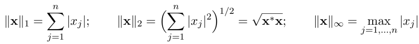
A vector is simply a column (or row) of numbers. We want to compare vectors in a convenient way. To do this we must aggregate the entries in the vector into a scalar number, and we use what we call norms to accomplish this. In theory there are an infinite number of ways to do this: according to this reference, there are three types of norms in most common use, they are as follows:

stadyn3norms — Left: the 1-norm. Center: the 2-norm, or Euclidean norm. Right: the infinity-norm.

So how do use norms in signal matching? We reduce the force-time (or in our case the velocity-time) history at the pile top after impact into a series of data points, and then for each point of time of each data point we compute the results our proposed model gives us and subtract it from the actual result. In the equation above each data point is a value $x_j$ . When we have all the differences in hand, we take them and compute a vector of differences, and then in turn take the norm of those differences. We do this successively by changing parameters until we get a norm value which is the minimum we can reach. For the STADYN program, we use the $\xi - \eta$ values as parameters and iterate using a polytope method (standard or annealed, for our test case the latter.)

For our purposes the infinity norm can be eliminated up front: in addition to having uniqueness issues (see Santamarina and Fratta (1998), we have enough of those already) it only concerns itself with the single largest difference between the two data sets. Given the complexities of the signal, this is probably not a good norm to use.

That leaves us with the 1-norm and 2-norm. To keep things from getting too abstract we should identify these differently, as follows:

1-norm = “Match Quality” for CAPWAP (see Rausche et. al. (2010))
2-norm = Least Squares or Euclidean norm (think about the hypotenuse of a triangle.) This relates to many methods in statistics and linear algebra, and has a long history in signal matching (Manley (1944).) This is what was used in the original study.

One thing that should be noted is that the norm we actually use is modified from the above formulae by division of the number of data points. This is to prevent mishap in the event the time step (and thus the number of data points) changes. However, for the Mondello and Killingsworth (2014) pile, the wall thickness of the steel section drove the time step, which did not change with soil changes; thus, this division is immaterial as long as it is done every time, which it was.

Application to Test Case

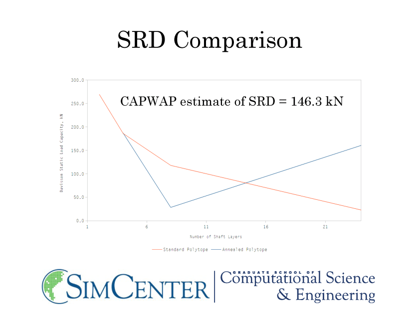
As noted earlier, we will use the four-layer case using the annealed polytope method of matching. Let us start at the end, so to speak, by showing the static load test data that the program runs with the final configuration:

Davisson Load, kN	Original $\nu$	$\phi$ -based $\nu$	% Change
1-norm	278	300	7.91%
2-norm	187.1	218	16.52%
% Change	48.58%	37.61%

The runs were done for both the original Poisson’s Ratio ( $\nu$ ) and that computed using the internal friction angle $\phi$ . The CAPWAP run done on this project recorded a Davisson simulated static load capacity of 146.3 kN.

Changing the way $\nu$ is computed produces larger variations in SRD (soil resistance to driving) for each of the norms than was evident in the last post. This is because the values of $\nu$ now vary with $\phi$ , which overall tends to increase the value of $\nu$ for the same value of $\phi$ . We will discuss this in detail below.

The most dramatic change took place with the norm was changed; the value for SRD is a third to a half higher with the Least Squares solution, depending upon the way $\nu$ is computed.

xi results
Layer	Original nu, 1-norm	Original nu, 2-norm	Phi-based nu, 1-norm	Phi-based nu, 2-norm
Shaft Layer 1	-0.708	-0.812	-0.686	0.471
Shaft Layer 2	-0.709	-0.751	-0.845	-0.96
Shaft Layer 3	-0.71	-0.984	0.966	-0.439
Shaft Layer 4	-0.586	0.428	-0.75	0.196
Pile Toe	-0.69	0.366	-0.491	0.804
Average	-0.681	-0.351	-0.361	0.014

The values of $\xi$ (degree of cohesion) tend to decrease for the Match Quality but the opposite for the Least Squares method. it is interesting to note that the Least Squares $\phi$ based $\nu$ is the only run to venture into predominately cohesive territory ( $\xi > 0$ , which is interesting in a soil which is generally characterized as cohesive.

eta results
Layer	Original nu, 1-norm	Original nu, 2-norm	Phi-based nu, 1-norm	Phi-based nu, 2-norm
Shaft Layer 1	-1.71	-0.622	-8.68	-1.08
Shaft Layer 2	-1.62	-1.38	3.29	-0.117
Shaft Layer 3	-0.838	-4.373	-1.86	-5.85
Shaft Layer 4	-1.74	-28.363	-14	-27.5
Pile Toe	-1.29	1.814	8.19	1.52
Average	-1.440	-6.585	-2.612	-6.605

The values of $\eta$ (consistency or density) are all low, but more so for the Least Squares cases than the Match Quality cases. Low values of $\eta$ are to be expected in a soil like this, but these tend to be extreme. Although limiters such as for elastic modulus are included to prevent serious misadventure in the soil properties, the existence of extreme values of $\eta$ is something that needs to be re-examined. ( $-1 < \xi < 1$ by physical necessity.)

Poisson’s Ratio Result
Layer	Original nu, 1-norm	Original nu, 2-norm	Phi-based nu, 1-norm	Phi-based nu, 2-norm
Shaft Layer 1	0.279	0.269	0.45	0.45
Shaft Layer 2	0.279	0.275	0.158	0.312
Shaft Layer 3	0.279	0.252	0.45	0.45
Shaft Layer 4	0.291	0.393	0.45	0.45
Pile Toe	0.281	0.387	0	0.45
Average	0.282	0.315	0.302	0.422

As was the $\eta$ values, the values of $\nu$ tend to increase with the $\phi$ based values. The Match Quality $\phi$ -based values are highly irregular, which in turn reflect the wide swings in $\eta$ with less cohesive values of $\xi$ .

Now let us present the optimization tracks for each of these cases.

The original study discusses the numbering system for the xi and eta parameters. In short, tracks 1-6 are for the shaft and 7-8 are for the toe. From these we can say the following:

The Match Quality runs tend to converge to a solution more quickly. The x-axis is the number of steps to a solution.
The Match Quality run tended to eta values that were more “spread out” while the Least Squares solution tended to have one or two outliers in the group.
The runs go on too long. This is because, in the interest of getting a working solution, the priority of stopping the run at a convergence was not high. This needs to be addressed.

Now the norms themselves should be examined as follows:

Final Norm	Original Nu	Phi-Based Nu	% Change
1-norm	0.148395682775873	0.134369614266467	-9.45%
2-norm	0.001494522212204	0.001456397402301	-2.55%

In both cases the difference norms decreased with the $\phi$ -based $nu$ , the Match Quality difference was more pronounced. The difference norm for the Match Quality is higher than the Least Squares solution, which is to be expected.

We finally look at the tracks compared with each other for the four cases.

It’s tempting to say that the Match Quality results “track more closely” but the whole idea of using a norm such as this is to reduce the subjective part of the analysis. However, this brings us to look at why one norm or the other is used.

The Least Squares analysis is widely used in analyses such as this. It is the basis for almost all regression analysis. However, the Match Quality has some advantages. It is considered more “robust” in that it is less sensitive to outliers in the data. In this case, the most significant outlier is the region around L/c = 1.5, which was discussed in the original study. Situations such as this reveal two sources of uncertainty in the model: the integrity of the mounting of the instrumentation, and the accuracy of the pile data (lengths, sizes, acoustic speed of the wood, etc.) The Match Quality certainly can help to overcome deficiencies caused by this and other factors. Whether this is at the expense of accuracy has yet to be determined.

So we are left with two questions:

If we were to improve the quality of the data by addressing the present and other issues, would we be better off if we used Least Squares? The answer is probably yes. Getting this in the field on a consistent basis is another matter altogether.
Will the two methods yield different results? With STADYN this is certainly the case; the use of the Match Quality with STADYN however yields results that are double those of CAPWAP. With CAPWAP we have no way of comparing the two; the Match Quality is all we have.

Conclusions

Based on all of this we conclude the following:

The use of a $\phi$ based $\nu$ leads to an improvement in the signal matching, due probably to the reduction in the number of real parameters being considered. It will probably remain as the default option.
Any final conclusions on this topic depend upon limiting the values of $\eta$ “within the box” to prevent serious outliers. This will be the topic of future study.
We also need to address the issue of stopping the runs at a more appropriate point.
The results for $\xi$ bring up again the question of the soil properties at the soil-pile interface vs. those in the soil body. We will discuss this in a later post.