This week we’ll turn in NAVFAC DM 7.2 to shallow foundations. It’s a well worn path and NAVFAC DM 7.2 does a good job covering it, but there are a points that are worth making. (Settlement for these foundations is covered in NAVFAC DM 7.1.)
Upper and Lower Bound Plasticity
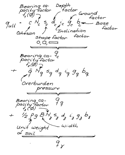
It’s mentioned in both NAVFAC DM 7.1 and NAVFAC DM 7.2 but not really explained: the whole concept of upper and lower bound plasticity. Until recently most American textbooks avoided the subject; I used Verruijt’s coverage of the subject, which had problems of its own but gave a reasonable introduction to the subject. NAVFAC DM 7.2 refers to Terzaghi’s bearing capacity method (which really needs to be retired from use) as an “upper bound” method, but the truth is that all of the bearing capacity methods mentioned–Terzaghi, Brinch-Hansen, Vesić (more about that shortly) and Meyerhof–are all upper bound methods. For a credible lower bound method which is good to illustrate the concept with bearing capacity, take a look at my post Lower and Upper Bound Solutions for Bearing Capacity.
Geotechnical Eccentricity
For both square/rectangular and circular foundations, this gets nice coverage, with illustrations, in NAVFAC DM 7.2. It’s a subject my students wrestled with, especially when juxtaposed with “middle third” types of distributions (and that’s covered too,) and this will be a help.
Vesić’s Method
If there’s one serious lacuna in the presentation on bearing capacity, it’s the lack of coverage of Vesić’s Method. That’s because the FHWA, for better or worse, has adopted it (or a modification of same) as their principal recommended method for bearing capacity.
Groundwater and Layered Stratigraphies for Bearing Capacity
The coverage of both of these topics is extensive and welcome. The groundwater part is basically the same method as the FHWA uses; the layered part is an advance over this or any other method I’ve seen. One question hangs over the festivities: what’s the best way to put them together?
Shallow Foundations on Slopes
This represents a major advance over the old book. My students found Meyerhof’s method hard to use (I did too) and the tabular alternatives given are a welcome break.
Mat Foundations
This is always a difficult topic because, at the end of the day, a computer solution is necessary for a realistic analysis. In the interim NAVFAC DM 7.2 furnishes a method which hopefully will be helpful for preliminary or verification work. One topic that isn’t consistently treated is whether a foundation should be analysed as rigid or flexible in the first place. NAVFAC DM 7.1 was very helpful when I put together When Semi-Infinite Spaces Aren’t, and When Foundations are Neither Rigid Nor Flexible, and a similar approach here would have been helpful.
The rest of the chapter focuses on drainage of shallow foundations and rock and soil anchors. The latter edges into deep foundations, which will be our next topic.
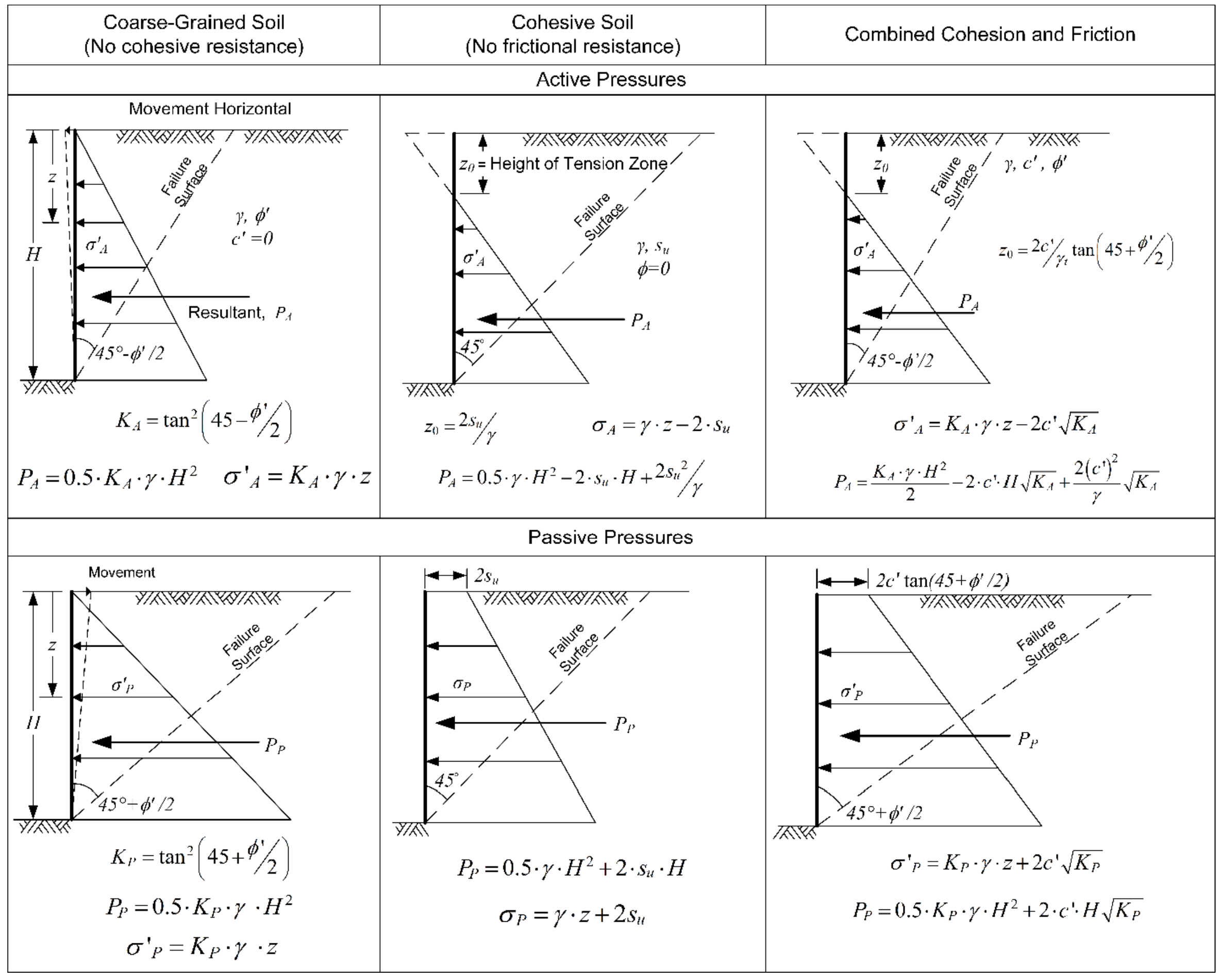
Now we get into a topic which has certainly been of interest to me, the co-author/editor of Sheet Pile Design by Pile Buck. I’m going to begin by tackling the subject of lateral earth pressure theories. NAVFAC DM 7.2‘s treatment of this subject is illuminating but raises many questions about how these relate to each other and to the design of retaining walls.
Acknowledging the Source of Jaky’s Equation
I’ll start with another topic, namely that of Jaky’s Equation, which is the “standard” for at-rest earth pressure theories. The first thing that comes up is the definition of the coefficient of earth pressure, given as
(4-1)
The hard truth here is that this is the definition of any lateral earth pressure coefficient; the difference is which theory is applied. It’s not just for at-rest earth pressures.
Turning to Jaky’s Equation, the equation for at-rest lateral earth pressure coefficients is given as
(4-2)
Obviously for normally consolidated soils (OCR = 1) this reduces to
but this is Jaky’s Equation, which is the basis for Equation (4-2). I think that credit needs to be given to its originator as has been the case with textbooks and reference books for many years.
Will the Real Rankine Theory Please Stand Up?
Now we get to the interesting part: the nature of Rankine Theory. The fact that, for vertical walls with level backfill and no wall-soil friction, the lateral earth pressure equations for both Rankine and Coulomb theory are the same. This has led to a good deal of confusion on the subject, such as “Rankine theory is just Coulomb theory with no wall friction,” but this is not the case. Rankine Theory is based on the application of Mohr’s Circle, while Coulomb Theory has its origins in static equilibrium of soil wedges. NAVFAC DM 7.2 does a good job making this distinction but in the process a few observations are in order.
First, while NAVFAC DM 7.2 goes into detail on the level backfill/vertical wall case, it does not include the “extensions” developed for sloping backfill. It states that “…there are published techniques that can accommodate inclined backfills.” I discuss one of these in my post Rankine and Coulomb Earth Pressure Coefficients. Excluding these restricts the use of Rankine theory in the same way we see in, say, Tsytovich, except that provision for cohesion is included.
Pursuant to that inclusion, NAVFAC DM 7.2 redraws this diagram from DM 7.02 in this way:
If they’re serious about making a clear distinction between Rankine and Coulomb theories, they need to eliminate the failure surfaces in the diagrams. I’m as aware as anyone of the role failure surfaces play in things such as anchor design, but it doesn’t change the basic nature of the theories. (I’m aware that there are rupture surfaces in Rankine theory, but they are different than wedge failure. Inclusion of a diagram such as is shown below (from this source) would have clarified the distinction.)
Finally, I don’t understand why they included the material on wall/soil interface friction angles in the section on Rankine theory, since Rankine theory doesn’t take into account wall/soil friction (it doesn’t consider soil/soil friction along a failure surface either.)
And as for Coulomb…
The presentation on Coulomb theory is similar to that in the old book with redrawn graphics and some tighter limits on acceptable limits of parameters such as wall friction and backfill angle. As was the case with the old book, NAVFAC DM 7.2 includes charts for vertical walls with sloping backfill and no wall friction for both the earth pressure coefficients and failure plane angle. And, like the old book, it doesn’t really explain why these charts are important. Should we ignore wall friction in many cases (the old book implied that we could for active pressures)? And how do the results of Coulomb theory under these conditions compare with the “Rankine extensions” with which the new book dispenses but are found in practice? (The answer to the last question can be found in the post Rankine and Coulomb Earth Pressure Coefficients.) I think that, with topics like this where there is significant variance in the way the theory is applied, DM 7 in general tends to “punt” on issues like these.
Coulomb earth pressure inevitably lead to the issue of trial wedge methods for complex geometries and stratigraphies. Personally I think that, with the advent of FEA, trial wedge methods are obsolete. NAVFAC DM 7.2 notes that “…finite element and finite difference soil structure interaction software can be used to solve these types of problems, but considerable skill is required to obtain meaningful results.” The same observation could be made about trial wedge methods. As someone who spent two decades in geotechinical education (and more if you include my work on this site) I don’t see the generation of engineers coming up developing the skill set for trial wedge methods.
Log-Spiral Methods
Log-spiral theory (especially in the passive case) has two significant advantages over Coulomb theory: it more accurately models the failure surface (FEA eliminates the need to do that, it figures it out for itself) and that in turn results in a smaller soil wedge and lower (less unconservative) earth pressure coefficients. Using these require a chart solution, and NAVFAC DM 7.2 makes a significant advance in that it abolishes the correction table for different values of and simply presents the chart for as a typical value. The new book expresses doubts about the accuracy of these correction factors, but there’s one thing for sure: it’s much less confusing and subject to error in use, and will make classroom teaching of this method much easier. My only concern about these is applying them to walls where soil/wall friction is minimal, as is the case with fibreglass and vinyl sheet piling.
The FHWA’s Solution
In its discussion of the log-spiral method, NAVFAC DM 7.2 states that (…passive pressure should be computed using the log spiral method and not the Coulomb method.” This is obviously due to the advantages of log-spiral methods discussed above. It’s worth noting (and the book should have done so) that the FHWA’s usual solution to this problem is to use Coulomb active/log-spiral passive combinations in practice, as they explain in the Soils and Foundations Reference Manual. This would have buttressed support for their case and given the engineer more definitive guidance in what can be a confusing topic.
Lateral earth pressure is the oldest analytic topic in geotechnical engineering; Coulomb published his paper in the same year the American colonies declared their independence from Great Britain. It is an indication of the nature of the field that we still do not have a firm consensus on how these are to be precisely computed and applied.
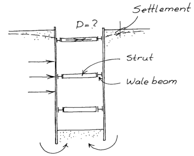
One of those “things” in geotechnical engineering that looks like “settled science” but may not be is the whole business of lateral earth pressures for braced cuts. (An example of one is shown at the right.) Textbooks of all kinds (including Soils in Construction) show pressure profiles and solution techniques that are “definitive.” Or are they? This article is more about asking questions than delivering another round of “definitive” answers, but hopefully it will at least spark some thought and perhaps make practitioners more careful in their application of these methods.
The Basic Problem
Based on experience, first in Berlin and later in Chicago, Terzaghi (and later also Ralph Peck) developed a set of pressure distributions as shown at the left. These are at variance with those usually associated with retaining walls in general and sheet pile walls in particular. The theory behind these (certainly for the clays) had its genesis in Rankine theory adapted for cohesive soils, but the distribution is rather different. These distributions have been reproduced in many textbooks and reference books, including Soils in Construction and Sheet Pile Design by Pile Buck.
It’s worth noting that there are other pressure distributions that have been formulated other than the ones shown above, as outlined by Boone and Westland (2005).
Along with the distributions came the method of using them: the “hinged method” of analysing the sheet pile wall. Strictly speaking the sheet pile wall is a continuous beam with multiple supports. Since there are usually more than two struts and supports, to use a continuous beam requires a statically indeterminate beam. Applying hinges (as shown at the right) can make the beam statically determinate. Although methods for solving statically indeterminate beams existed in Terzaghi’s day (remember it was geotechnical methods which then and now lag the rest of civil engineering in advancement,) converting the problem to a statically determinate one was convenient for computational purposes.
But then comes the kicker: as generally presented, if the distributions above are used, they must be used with the hinged method, even when analysing a braced cut wall using a braced cut method with a continuous beam is nearly trivial now. Why is this?
How It Came About
Like so many things in civil engineering, the investigation of pressures on braced cuts came about as a result of tragedy. As noted by Rogers (2013):
On the evening of December 1, 1938 Terzaghi delivered a terse lecture titled “The danger of excavating subways in soft clays beneath large cities.” The lecture focused on his recent experiences with construction of the Berlin Subway, which was hampered by a high water table in running sands. These conditions had contributed to the sudden failure of a shored excavation which killed 20 workers in August 1935. He made a convincing case for proper geotechnical oversight during construction if similar tragedies were to be avoided in Chicago.
The lecture with its graphic images of the dead bodies beneath the collapsed bulkhead along the Hermann Goring Strasse succeeded in scaring his audience to death, and promptly found the State Street Property Owners’ Association and City of Chicago bidding for Terzaghi’s services. The City wanted him to advise them on how best to monitor progress of excavations and ground settlement, differentiating what structural or architectural damage was caused by subway construction.
One might ask, “How did they come up with the earth pressure distributions?” They did so–and this is the key to the problem–by measuring the reactions on the braces. They did this in the face of the fact that, as is usual with braced cuts, the braces were put in successively with excavations, and that much of the movement of the wall–and thus the mobilisation of the earth pressures–was in place before the braces were installed. (It is easy to forget the importance of that mobilisation, but both Terzaghi and Peck were well aware of it and its effects.) To translate the loads on the braces into a pressure distribution, they adopted Terzaghi’s procedure from the Berlin subway as follows (Peck (1943)):
The vertical members of the sheeting are assumed to be hinged at each strut except the uppermost one, and a hinge is assumed to exist at the bottom of the cut. The abscissas of the pressure diagram “A” represent the intensity of horizontal pressure required to produce the measured strut loads. A study of such diagrams for all of the measured profiles disclosed that the maximum abscissa never exceeded the value KA Ya H. Every measured set of strut loads resulted in a different pressure diagram “A,” all of which were found to lie within the boundaries of the trapezoid indicated by the dotted lines. Thus, if strut loads are computed on the basis of this trapezoid, they will most probably be on the safe side.
This, therefore, is the origin of the requirement to use a hinged wall where there were no actual hinges. At the time it was a reasonable solution. As noted earlier, solutions for continuous beams existed but back-figuring the pressures using them would have been a formidable “inverse problem” given the computing power of the day. Doing this, however, raises as many questions as it answers, such as the following:
If a continuous beam had been used, would the pressure distribution have been different?
What is the relationship between the pressure distribution computed by Terzaghi’s method and what is actually experienced by the wall? Put another way, did Terzaghi’s simplification of the structural situation compromise his distribution? (No doubt some conservatism in the pressure distributions offset that problem.)
If the pressure distributions are right for engineering purposes, is it still necessary to use a hinged solution? Especially with beam software, a continuous beam is much simpler to analyse and structurally more representative of the actual sheeting and bracing.
Peck himself was well aware of the limitations of the method; he made the following admission:
It is apparent, therefore, that it is useless to attempt to compute the real distribution of lateral pressure over the sheeting. Of far greater practical importance is the statistical investigation of the variation in strut loads actually measured, in order to determine the maximum loads that may be expected under ordinary construction procedures.
This too raises another question: in developing distributions primarily to determine brace/strut loads, do we compromise the accuracy of determining the maximum moment in the sheeting itself?
Moving Forward
It’s difficult to really know how to answer many of the questions this problem raises. Some suggestions are as follows:
It is hoped that there is enough conservatism in these earth pressure distributions to accommodate either method. That’s likely, as inspection of some of Peck (1943) curves will attest. That likeliness is buttressed by the fact that these methods came out of a deadly accident.
More comparisons of hinged and continuous beam models are needed. There is one in Sheet Pile Design by Pile Buck and another in the post on this site A Simple Example of Braced Cut Analysis. These are simply not enough to establish a trend one way or another, although the results are interesting and hold promise.
A “hand” solution based on parametric studies using FEA or another numerical method would move things forward considerably. Obviously these are limited by the accuracy of the soil modelling but they can be applied to a wider variety of cases.
Field tests should include measurement of actual lateral earth pressures on the sheeting at various points. The use of strut loads, although easier to measure with the technology of the 1930’s and 1940’s, is still indirect. Another interesting approach is to use an inverse method and a continuous beam with existing data, although this is not as satisfactory as direct measurement of earth pressures.
References
Boone, S.J. & Westland, J. (2005) “Design of excavation support using apparent earth pressure diagrams: consistent design or consistent problem?” Fifth International Symposium on Geotechnical Aspects of Underground Construction in Soft Ground, International Conference on Soil Mechanics and Geotechnical Engineering, 809 – 816.
Peck, R.B. (1943) “Earth-Pressure Measurements In Open Cuts, Chicago (Ill.) Subway.” Transactions of the American Society of Civil Engineers, Vol 108, pp 1008-1036.
Last year I posted The Sorry State of Compression Coefficients where I a) gave a brief summary of earlier posts on consolidation settlement and b)showed that there was more than one way to express them. An example of the “alternative” (for geotechs in some countries it’s the accepted way) compression coefficient is “Hough’s Method” which is featured in both the Soils and Foundations Reference Manual and the Shallow Foundations manual. Hough’s Method, however, is for cohesionless soils. Why, you ask, can methods usually associated with cohesive soils be applied to cohesionless ones? Because consolidation settlement methods using the logarithmic difference of pressure reflect the fact that the elastic (or shear) modulus of a soil increases as the void ratio/porosity of the material decreases, which I discuss in From Elasticity to Consolidation Settlement: Resolving the Issue of Jean-Louis Briaud’s “Pet Peeve”.
In this post I will attempt to do two things:
The method as presented in the above references has been described as too conservative, i.e., the settlements predicted are too large. I will attempt to explain this and perhaps offer a solution based on Hough’s own works.
Discuss the whole business of bearing capacity vs. settlement failure in shallow foundations, which was perhaps the greatest legacy of Hough’s work and remains an important issue in geotechnical engineering today.
Bearing Capacity vs. Settlement
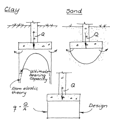
Terzaghi’s solution (or more accurately his adaptation of Prandtl’s punching shear theory) of the bearing capacity problems was one in a number of solutions that became “reference standard” in geotechnical engineering.
We were regaled with photos of Canadian grain elevators on their side to show that bearing capacity failure was the first thing we should look for in shallow foundation design. Terzaghi’s formula was so highly regarded that for many years it was fashionable for introductory geotechnical courses to require students to learn both Terzaghi’s method and the subsequent improvements/extensions of that method by researchers such as Meyerhof, Vesic, Brinch Hansen, etc..
Up until that time shallow foundations were generally designed using what we call “presumptive bearing capacities” based on soil types and foundation configurations. These were enshrined in the building codes of the day. They were generally purely empirical in nature, as was most of geotech in the era before Terzaghi and his contemporaries. They had one advantage however: because they were derived from actual performance, be it ever so crude, they included the effects of soil settlement under load.
Like any other engineering material, only on a larger basis (because their elastic/shear moduli were several orders of magnitude lower than more conventional materials) soil is deformable under load. That deformation not only allows the foundation to deflect under load, it also affects the failure surfaces as they develop. The latter reality became apparent and so we have the modification of the bearing capacity for punching and local shear. It should be noted that Terzaghi and Peck were well aware of the problem of settlement, and included provision for it in their classic 1948 textbook Soil Mechanics in Engineering Practice.
One possible solution was to use elastic theory for the initial settlement. The implementation of that is discussed in Analytical Boussinesq Solutions for Strip, Square and Rectangular Loads. It is even possible to develop a lower bound solution for the bearing capacity problem, as was discussed in Lower and Upper Bound Solutions for Bearing Capacity. The problem with this is twofold. The first is that the lower bound solution assumes that the footing is a purely flexible foundation, which is not really true with this type of foundation. The second is that, if we went to the other extreme and assumed a purely rigid foundation, by elastic theory the stresses at the corners is infinite for any load. (This is conventionally attributed to foundations in cohesive soil, but it can be shown to be true by elastic theory.)
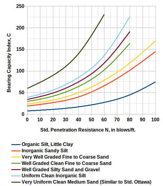
Hough’s Settlement Method
Hough presented his settlement method in his 1959 ASCE paper. He starts by presenting a graph similar to the following, which illustrates the transition from small, elastic displacement to large inelastic ones:
The solution is in the form (similar to that presented in Verruijt) of
The coefficient is determined using a chart which is below.
The chart itself is basically the same as the one in Hough (1959,) but now things get complicated.
Cheney and Chassie (2000) recommend that the SPT blowcounts be corrected for overburden pressure before correlating the N-values to the bearing capacity index, C′. An overburden correction by Bazaraa (1967) was recommended by Cheney and Chassie (2000). Since that time, many researchers have studied the effect of overburden stress on the SPT N-value, largely in support of liquefaction hazard assessment procedures. Recent consensus by the 1996 and 1998 National Center for Earthquake Engineering Research (NCEER) (Youd et al., 2001) concluded that the correction proposed by Liao & Whitman (1986) (shown in Figure 5-18) could be used for routine engineering applications. Therefore, the correction by Liao & Whitman is included here as part of the Hough procedure, in particular because it is easy to calculate and can be used without charts in simple computation spreadsheets.
The basic problem with this is that Hough himself never mentions any kind of correction for the variations of the SPT tests, overburden or otherwise, and that in modifying Hough’s Method we run the risk of making some assumptions that may not be applicable.
The idea of using the SPT tests, even with shallow foundations in cohesionless soils such as the ones Hough is concerned about, is admirable on the face because undisturbed samples of these soils are hard to obtain in normal soil testing. The problem with SPT tests–which were coming into acceptance when Hough presented his original method–is that their variations in both configuration and those induced by the overburden are significant. It wasn’t until the 1980’s that this was “formally” sorted out with the correction system that we have today.
With our current method we have two stages of correction. The first stage is for variations in the configuration of the split spoon, the effect of the rod and borehole, and most importantly the efficiency of the hammer itself. The second is for the overburden. In both his original paper and the presentation of the method in the Second Edition of his textbook Basic Soils Engineering (1969,) Hough does not delve into either of these.
The whole point of the N60 correction (the first series) was to harmonise the results to a single mechanical standard, and one that was generally attained “back in the day” so that empirical methods such as Hough’s could be used today. We could assume that Hough’s value are at least N60 values, although we’re not guaranteed of that due to the lack of supporting data.
The business of overburden correction brings up Bazaraa (1967.) At this point credit needs to be given where credit is due: Bazaraa had the thankless task of sorting out the settlement methods which were current in his day, and that task included dealing with the variations of the SPT method. Since his overburden correction method was originally used with Hough’s Method and then changed, let us compare the two. We start be defining
The two correction factors for overburden are shown below.
Except for the region where Liao and Whitman is “flat topped” the two are reasonably close, and so substituting Liao and Whitman’s correction is legitimate, assuming it should be used at all.
It should be noted, however, that Bazaraa’s objective is not to correct Hough’s method, which he did not do: it was to provide a new method of estimating settlements in cohesionless soils, and to advance Terzaghi and Peck’s 1948 method. So we are still “up in the air” about how to apply all of this to Hough’s Method.
If the overburden stress is less than the standard atmospheric pressure (approx. 2 ksf) then the N value used will be increased, the C’ values will likewise increase, and the estimated settlement will decrease, which may be more accurate but moves away from conservatism. If the opposite is true then the result will be more conservative. For shallow foundations such as Hough’s Method the lower overburden stresses will be more of a factor (depending upon the depth D.) At this point it is not clear to me (at least) that including an overburden correction is really significant given the other unsolved problems that exist with this method.
One further complicating factor is that, in the aforementioned Second Edition of Basic Soils Engineering, Hough presents a new chart (again with no explanation of correction of any kind) which is redrawn as follows:
Very Uniform Clean Medium Sand (Similar to Std. Ottawa)
58.66
0.0225
It should be noted that, where the curves are directly comparable with Hough (1959), they tend to be lower, i.e., the values of C are less. This would increase settlement and thus conservatism. At this point perhaps we should consider Hough’s Methods in the plural rather than the singular.
We have the conventional Cc based on either liquid limit, initial void ratio or water content. Hough is represented here as well; however, these correlations are for cohesive soils. Hough himself had a broader application for these.
In the Second Edition of Basic Soils Engineering, he presents a function to compute Cc as follows:
He also establishes a relationship between correlations based on liquid limit and those on void ratio, but getting to that is for another time.
In any case he presents values for this equation which are tabulated below, and include both cohesionless and cohesive soils.
a
b*
Uniform cohesionless Material (Cu < 2)
Clean Gravel
0.05
0.5
Coarse Sand
0.06
Medium Sand
0.07
Fine Sand
0.08
Inorganic Silt
0.1
Well-graded, cohesionless soil
Silty sand and gravel
0.09
0.2
Clean, coarse to fine sand
0.12
0.35
Coarse to fine silty sand
0.15
0.25
Sandy silt (inorganic)
0.18
0.25
Inorganic, cohesive soil
Silt, some clay; silty clay; clay
0.29
0.27
Organic, fine-grained soil
Organic silt, little clay
0.35
0.5
*The value of the constant b should be taken as emin whenever the latter is known or can conveniently be determined. Otherwise, use tabulated values as a rough estimate.
From here we can use the well-tried “Cc” formulae (which would include preconsolidated soils) to estimate settlement. This opens up a new vista for using conventional consolidation settlement theory to estimate the settlements of cohesionless soils.
To return to our original objectives, settlement and bearing capacity are, in the process of failure, two sides of the same thing. It is also worth noting that most foundations fail in settlement, although the failure isn’t as “spectacular” as bearing capacity.
The only way to treat them together is to use a method that can combines both phenomena, and finite element methods are capable of doing that. However our profession has been uncomfortable with “black box” methods such as these, although they really apply the same laws we use to formulate closed form solutions. In that respect they have value, and to apply methods such as Hough’s to cohesionless soils with better calibration of the constants would be a good step forward.
References
Bazaraa, A.R.S. (1967). “Use of the Standard Penetration Test for Estimating Settlements of Shallow Foundations on Sand,” Ph.D. Thesis presented to University of Illinois, Urbana.
Hough, B.K. (1959). “Compressibilty as the Basis for Soil Bearing Value,” Journal of the Soil Mechanics and Foundations Division, ASCE, Vol. 85, Part 2.
Hough, B.K. (1969). Basic Soils Engineering. Second Edition. New York: Ronald Press Company.
This is the last (hopefully) post in a series on consolidation settlement. We need to start by a brief summary of what has gone before. Note: the material for this derivation and those that preceded it have come from Tsytovich with some assistance from Verruijt.
where E is the modulus of elasticity and is a factor based on Poisson’s Ratio and includes the effects of confinement, be that in an odeometer or in a semi-infinite soil mass. We also showed that, for a homogeneous layer,
(2)
where is the settlement of the layer, is the thickness of the layer and is the uniaxial stress on the layer. The problem is that is not constant, and the settlement more accurately obeys the law
(3)
where is the compression index, is the initial void ratio of the layer, is the change in pressure induced from the surface, and is the average effective stress in the layer.
Turning to the post Deriving and Solving the Equations of Consolidation, we first determined that the change in porosity could, for small deflections, be equated to the change in strain . From this we could say that
(4)
The change in porosity, for a saturated soil whose voids are filled with an incompressible fluid (hopefully water) induces water flow,
(5)
where is the flow of water out of the pores and is the porosity as a function of position and time. The flow of water is regulated by the overall permeability of the soil, and all of this can be combined to yield
(6)
where is the permeability of the soil and is the unit weight of water. Defining
(7)
and making some assumptions about the physics, we can determine the equation for consolidation as
(8)
where $latex u(x,t) is the pore water pressure. If we invoke the effective stress equation and solve this for the boundary and initial conditions described, we have a solution
(9)
The Degree of Consolidation
One thing that our theory presentation demonstrated was the interrelationship between pore pressure, stress and deflection. We know what the ultimate deflection will be based on Equation (3) above (or more complicated equations when preconsolidation is taken into consideration.) But how does the settlement progress in time?
We start by defining the degree of consolidation thus:
(10)
where is the settlement at any time before complete settlement. For the specific case (governing equations, initial equations and boundary conditions) at hand, the degree of consolidation–the ratio of settlement at a given point in time to total settlement–can be determined as follows:
(11)
In this case the result is divided by the uniform pressure p and the height h. Let us further define the dimensionless time constant
(12)
That being the case, if we integration Equation (9) with Equation (11), we obtain
(13)
otherwise put
(14)
As was the case with Equation (9), only the odd values of n are considered; the even ones result in zero terms.
It is regrettable that, in defining , the value was not included, as using Equation (14) would be much simpler. For certain cases, it is possible to use the first two or three terms. In any case the usual method for determining –and by extension the degree of consolidation–is generally done either using a graph or a table, as is shown in the graph at the start of the post (repeated below:)
Degree of Consolidation for Instantaneous Uniform Loading and One-Dimensional Flow. From NAVFAC DM 7.1: Soil Mechanics
The notation is a little different. We use the variable to emphasise that we are dealing with the “standard” case. The above graph also gives approximating equations; it is easy to see that, for , the equation given is simply the first two terms of Equation (14). The distinction between the drainage length h ( in the graph above) and the layer thickness H is clear.

 (4-1)
(4-1) (4-2)
(4-2)

 and simply presents the chart for
  as a typical value. The new book expresses doubts about the accuracy of these correction factors, but there’s one thing for sure: it’s much less confusing and subject to error in use, and will make classroom teaching of this method much easier. My only concern about these is applying them to walls where soil/wall friction is minimal, as is the case with fibreglass and vinyl sheet piling.
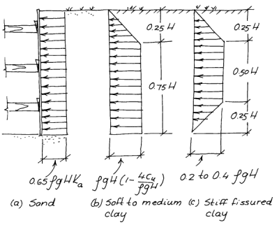


 is determined using a chart which is below.
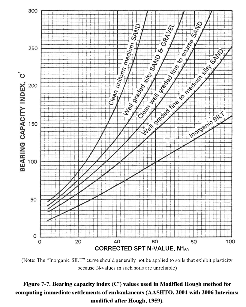

 for overburden are shown below.
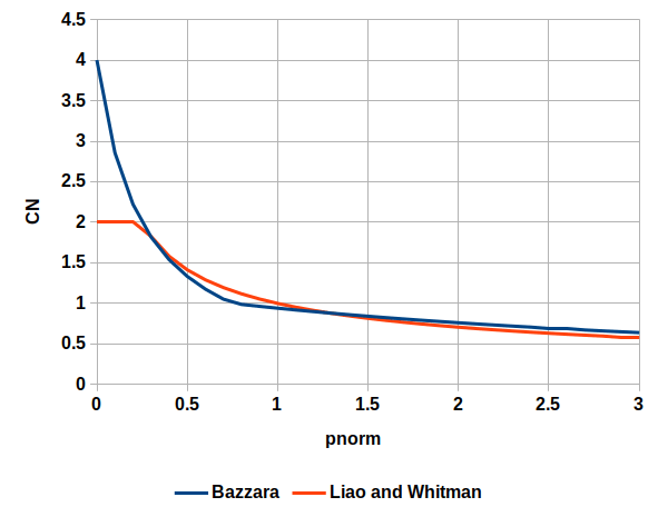


 by
by (1)
(1) is a factor based on Poisson’s Ratio and includes the effects of confinement, be that in an odeometer or in a semi-infinite soil mass. We also showed that, for a homogeneous layer,
 (2)
(2) is the settlement of the layer,
  is the thickness of the layer and
  is the uniaxial stress on the layer. The problem is that
  (3)
(3) is the compression index,
  is the initial void ratio of the layer,
  is the change in pressure induced from the surface, and
  is the average effective stress in the layer.
 could, for small deflections, be equated to the change in strain
  . From this we could say that
 (4)
(4) (5)
(5) is the flow of water out of the pores and
  is the porosity as a function of position and time. The flow of water is regulated by the overall permeability of the soil, and all of this can be combined to yield
 (6)
(6) is the permeability of the soil and
  is the unit weight of water. Defining
 (7)
(7) (8)
(8) (9)
(9) (10)
(10) is the settlement at any time before complete settlement. For the specific case (governing equations, initial equations and boundary conditions) at hand, the degree of consolidation–the ratio of settlement at a given point in time to total settlement–can be determined as follows:
 (11)
(11) (12)
(12) (13)
(13) (14)
(14) , the value
  was not included, as using Equation (14) would be much simpler. For certain cases, it is possible to use the first two or three terms. In any case the usual method for determining
  to emphasise that we are dealing with the “standard” case. The above graph also gives approximating equations; it is easy to see that, for
  , the equation given is simply the first two terms of Equation (14). The distinction between the drainage length h (
 in the graph above) and the layer thickness H is clear.