the page with geotechnical engineering resources and educational materials
Category: Geotechnical Engineering
Fugro defeated 60 other teams from industry and academia in a contest to predict pile driving blowcount vs. depth for jacket piles installed in the North Sea. The contest ran from April to December of […] The post Fugro Wins Pile-Driving Prediction Contest With Machine-Learning appeared first on GeoPrac.net.
Note: since this was originally posted, it has been extensively revised. There are better ways of presenting this information than are given in most American geotechnical textbooks and hopefully you will agree.
Students and practitioners alike of geotechnical engineering have learned and used Boussinesq elastic solutions for stresses and deflections induced in a semi-infinite space by structures at the surface. Although these solutions are very idealized and have many limitations, they’re still useful.
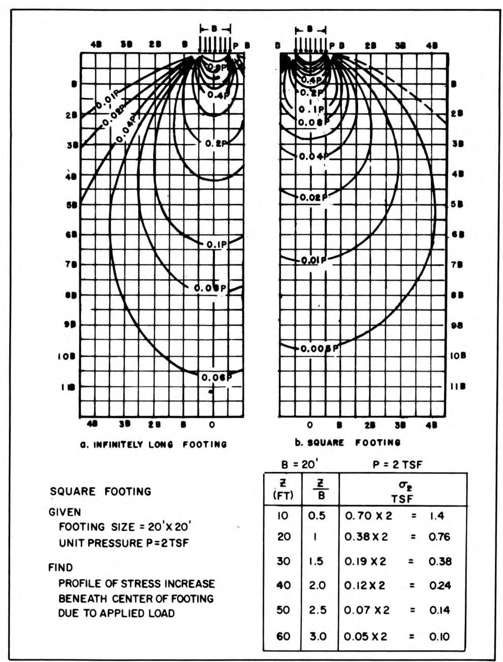
For the most part engineers have implemented these solutions–especially for loads other than point or line loads–using charts. This chart, from Naval Facilities Engineering Command (1986)–DM 7.01, Soil Mechanics, shows the isobars for stresses induced by strip and square foundations.
In addition to being hard to read (a fault which has been fixed in many of the books that have cribbed this chart) it requires a great deal of interpolation to use it and many others. In the past, the computational demands of using analytical solutions put them out of reach for practical use and educational purposes. That’s no longer the case; however, some of those solutions are difficult to find. This piece attempts to bridge that cap and set forth analytical solutions that can be used, along with a spreadsheet to implement at least some of them.
Assumptions of the Solutions Presented
They assume that the load is applied to a linear elastic, homogeneous semi-infinite space.
They assume that the foundation is completely flexible; rigid (or intermediate foundations) are not considered.
They do not consider strain-softening hyperbolic effects. These are extensively discussed in this monograph. It is more than likely that, for the cases presented here, a homogenized value for the modulus of elasticity can be arrived at, perhaps by using the methods used in the linked monograph for the toe.
Principally the vertical stresses will be considered.
All of the loads on the foundation are uniform.
Stresses Under Strip Loads
The simplest case for this set of foundation geometries is the strip load, which reduces a three-dimensional problem to a two-dimensional one. The problem is illustrated (and a point under consideration located) in the figure below, modified from Tsytovich (1976).
Diagram and Variables for Strip Load Problem, from Tsytovich (1976)
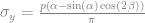
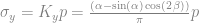
where is the uniform pressure on the foundation in load per unit area, and is the width of the foundation, usually expressed in American practice as . The angles are as shown. The stresses are as follows:
If we rewrite these equations thus
we thus have defined three influence coefficients (the “K” variables) which we can use to generalise the results.
Given the foundation width or and the angle , any point in the half space can be defined. They can be related to the Cartesian coordinates as follows:
At the base of the foundation, and , which means that the soil stress is equal to the foundation pressure , as we would expect. The stress is zero at the surface away from the foundation.
The tricky part of this is in determining from the geometry of the system and the desired location of the point in question. For students, probably the simplest way of doing this is to use CAD software. Alternatively we could also directly compute the stress from the z and y coordinates directly; for the vertical stresses only,
For stresses under the foundation centre, this influence coefficient can be reduced to
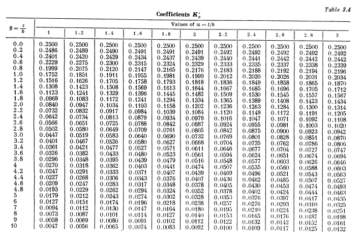
All three influence coefficients can be computed and tabulated in general. Using the two coordinate ratios and , the tabulation of these coefficients is shown below.
Influence Coefficients for Determination of Component Stresses for the Strip Load Problem (from Tsytovich (1976))
A couple of interesting graphics can be shown from these relationships.
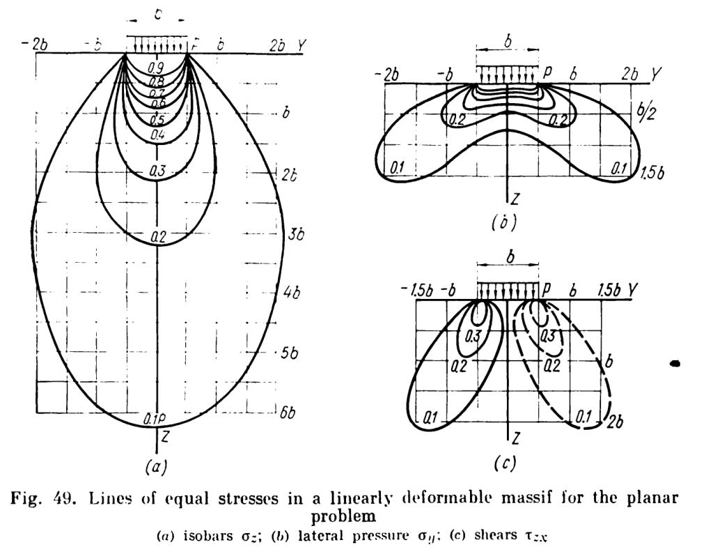
The first is the graphical representation of the tabular data of the table above, shown below.
Graphical Representation of Stresses under a Strip Load, from Tsytovich (1976)
It is interesting to note that, at the centre axis under the load, the z-direction stresses are at their maximum as a function of depth. The shear stresses along that axis are zero, and are at their maximum under the edges.
Another interesting graphical representation are the stress ellipses, whose major and minor axes denote the principal stresses. These always are along the line of the angle , not necessarily to the centre of the foundation.
Stress ellipses under a strip load, from Tsytovich (1976)
The elastic stress computations can be used to estimate the lower bound permissible stresses for bearing capacity failure, as is shown here. The direction of the principal stresses is an important part of that derivation.
Stresses under Square and Rectangular Loads
These are well known, and most engineers and engineering students have used the “Fadum charts” as shown below to obtain the solution.
Both the strength and the weakness of the charts is that the stresses computed are under the corner of the rectangle/square. It is a very specific position, but by using superposition (permissible with elastic, path-independent solutions) we can add and subtract rectangles to obtain the stress at just about any point under or near the structure in question.
Another weakness of the Fadum chart, however, is that it’s hard to read. Fadum made the results dimensionless in such a way that m and n are interchangeable, which is certainly justified by the theory, but dispensing with that can make for a solution that is easier to read. Now, of course, the increase in computational power makes use of the equations that generated the Fadum chart more accessible, but for everyday work a solution that allows for either is the best.
Bowles (1996) presented the solution that has been most widely disseminated, but ultimately most solutions are based on that of Newmark (1935). His solution was as follows:
where B, L and Z are the width, length and depth of the point of interest below the corner.
Let us, following Tsytovich (1976), define three different dimensionless variables thus:
(the influence coefficient for the vertical stresses)
(the aspect ratio of the foundation or the part of the foundation of its length (longer side) divided by its width (shorter side)
the aspect ratio of the foundation or part of the foundation of the depth from the corner to its shorter side.
As was the case with Bowles (1996), which equation you actually use depends upon what quadrant the second (arcsin or arctan) term ends up in. The equations using these dimensionless variables are as follows:
If :
If :
The “border” between the two equations is shown below.
Plot of Curve where the form of the equations change.
A table representing the results is below.
The biggest drawback to this is that the sides aren’t as interchangeable as with the Fadum charts, but since for rectangles L>B customarily that shouldn’t pose much of a problem.
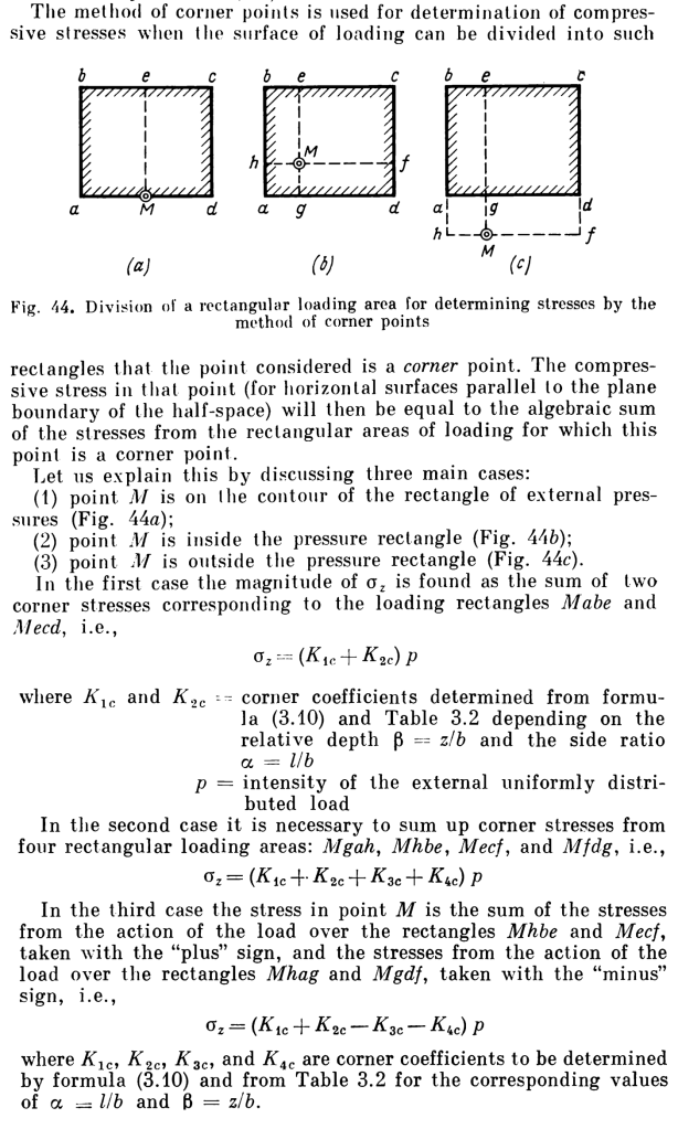
Obviously we might be interested in points below the surface other than those directly under the corner. This can be done using superposition (which is available since all of this is elastic theory and thus the results are path independent.) Below is a description of how it is done, using charts with a plan view of the foundations:
Method of using superposition to determine the vertical stress at a point under a foundation at a point other than a corner. Note that all of the K factors can be determined using Table 3.4 above. From Tsytovich (1976)
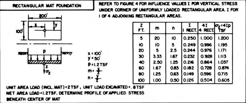
As an example of Case (b), consider determining the stress in the centre of the foundation, as is the case in this example, from NAVFAC DM 7.01:
This problem was solved using the Fadum Chart. To use the method shown, we simply need to realign our variables. For the stresses at the centre, the foundation being analysed is one fourth of the original. So we set L = 100′ and B = 50′, which means that . The values for are shown as follows:
Z
5
0.1
10
0.2
20
0.4
30
0.6
40
0.8
60
1.2
80
1.6
100
2
The influence coefficients can be determined either by the equations or the table. They should be identical to those shown in the example; however, since those were probably taken off the chart, there will be small variations. Once they are determined, they should be multiplied by 4 for the complete solution.
It is interesting that the problem reduces the net pressure on the foundation by the effective stress at the base of the foundation. This is one way to deal with this problem; it is used in Schmertmann’s Method for settlement. You need to look at how you plan to use the results before doing this. It is important to note, however, that no matter how you handle this the value of Z is the distance from the base of the foundation, not the surface of the soil.
Diagram for problem where there are two different pressures and two different foundations, from Verruijt (2007)
It should be noted that adding the influence coefficients K assumes that the p is the same for the whole foundation. The method can be expanded to foundations where that is not the case and an example of this is given in the Rectangular Elastic Solutions Spreadsheet, featuring a problem taken from Verruijt, A., and van Bars, S. (2007). Soil Mechanics. VSSD, Delft, the Netherlands., who solve the problem using Newmark’s Method. The difference is that, while the description from Tsytovich adds K factors, the problem here adds and subtracts stresses. Using the formulae the superposition method is more precise than Newmark’s Method.
Another description of the superposition method, from NAVFAC DM 7.01 (1986)
Deflections of Squares and Rectangles
Elastic solutions can be used to predict both stresses and deflections. Most engineers are familiar with tables such as this, and these are still used for initial deflections and deflections in media such as intermediate geomaterials (IGMs.)
Keeping in mind that we are still assuming the foundation to be perfectly flexible relative to the soil/IGM/rock, the equation for the deformation of the foundation is as follows:
where
settlement of the foundation at the point of interest
influence factor, given in the table below
uniform pressure on the foundation
smaller dimension of rectangle or dimension of square side
Poisson’s Ratio of the soil
Modulus of elasticity of the soil
The factors are given below, both for a soil layer of large depth and one of limited depth .
Table for Values of Influence Coefficients, from Tsytovich (1976)
The table also includes values for rigid foundations, which we will not consider here.
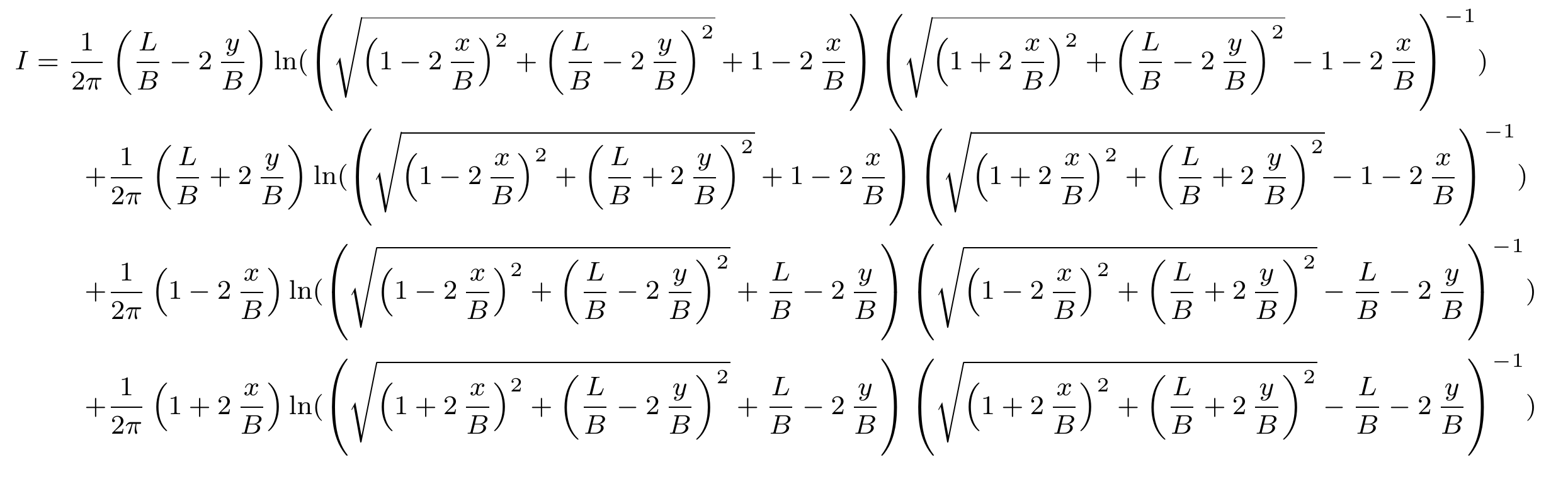
As was the case with the stresses under square or rectangular foundations, the equations for the deflections are quite involved. For these foundations, assumed flexible and uniformly loaded, the influence coefficient is computed by the following equation (Perloff and Baron, 1976):
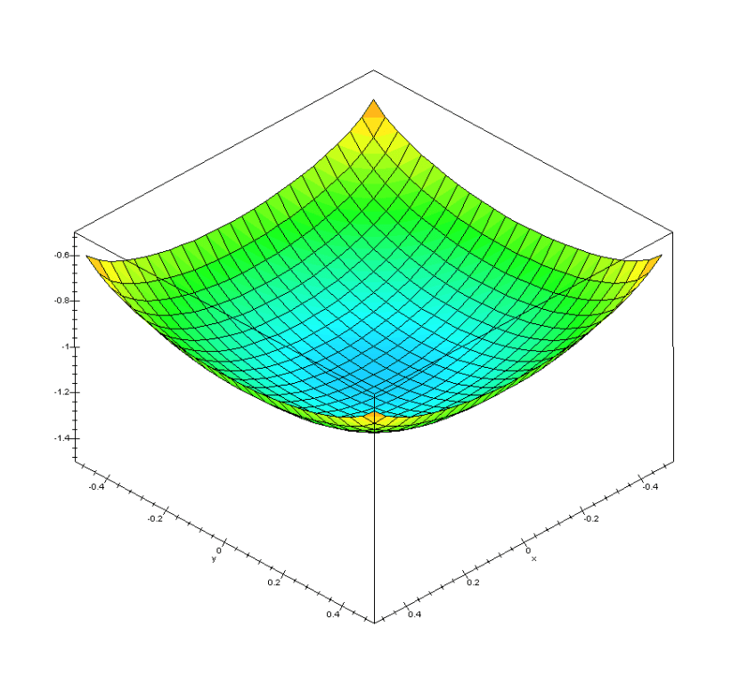
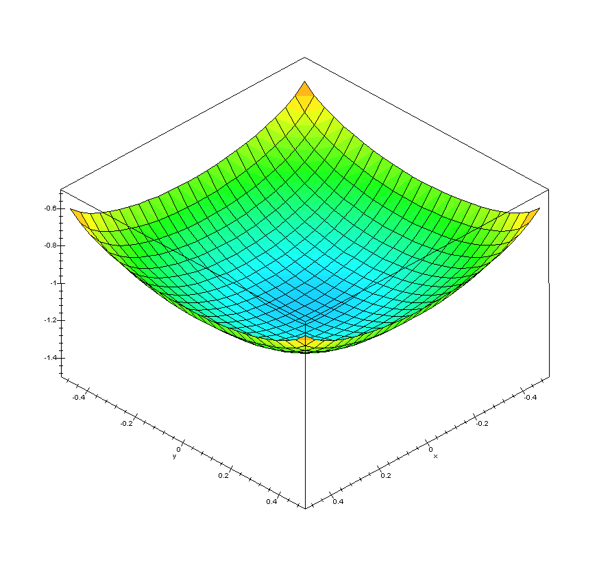
In this equation the origin is assumed at the centre of the foundation, not at the corner. Thus, the values of x and y are as follows: -B/2 < x < B/2 and -L/2 < y < L/2. As an example of how this looks over an entire foundation, consider the case of B=L=1 (a square foundation.) The influence coefficient of the foundation can be plotted as follows:
It is easy to see what is meant by “flexible” foundation.
The problem with this formula is that, if blindly followed mathematically (just inserting the variables) singularities quickly arise both along the edges or at the corners. Symbolically solving (and taking a few limits) get around this. For the mid-point of the edges,
And at the corners,
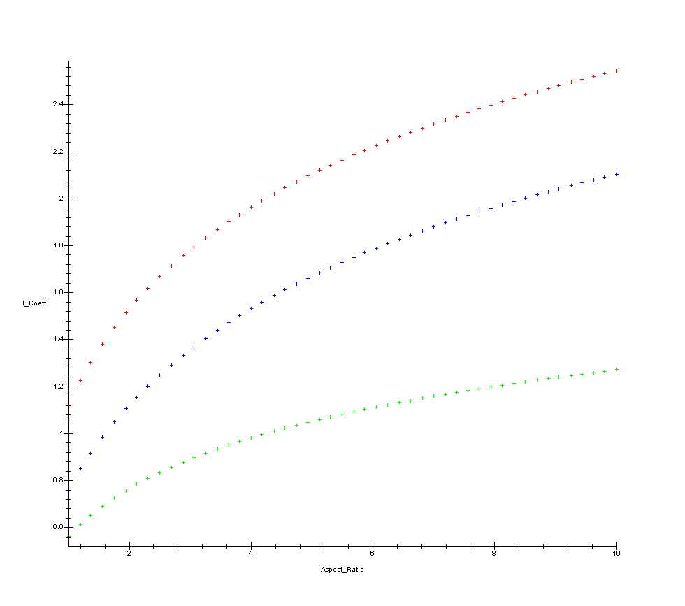
A plot of the same functions mentioned in the table above from the formulae is below.
Rectangular foundation deflection for the center (red,) mid-point of the long side (blue,) and corner (green) for various aspect ratios of L/B
The center deflection can be found by either substituting x=0, y=0 into the first equation or by using the equation
Some Observations
Use of theory of elasticity in this way has been employed in foundation design for a long time, even with the inherent limitations of the method. It gives reasonable approximations for either initial deflections or for deflections of IGM’s. For implementation on a recurring basis, use of the formulas allows a more precise implementation of these methods but not necessarily a more accurate one, but the errors inherent in reading charts are eliminated.
In our opinion it is possible to improve the accuracy of the method by improving our understanding of the elastic modulus of the soil, and in particular strain-softening near the foundation itself.
The deflections are probably the less satisfactory products of this theory than the stresses. No foundation is either purely flexible or rigid, and using a purely flexible foundation produces larger variations in deflections than one would expect in reality. Also, the typical rule of thumb that foundations with an aspect ratio larger than 10 can be treated as continuous/infinite foundations is reasonable for stresses but not for deflections, and in fact the chart shown above was truncated. Whether this is reflected in reality is another question, and this too doubtless relates to the flexibility of the foundation.
Other References
Bowles, J.E. (1996) Foundation Analysis and Design. Fifth Edition. New York: McGraw-Hill.
Perloff, W.H., and Baron, W. (1976) Soil Mechanics: Principles and Applications. New York: Ronald Press.
Most retaining walls are designed with active or passive earth pressures derived from Rankine, Coulomb or Log-Spiral theories. One notable exception to that are braced cuts. The development of the earth pressure distributions is attributable to Karl Terzaghi and Ralph Peck, a process outlined in the post Getting to the Bottom of Terzaghi and Peck’s Lateral Earth Pressures for Braced Cuts. In the process of developing those, the way the wall is modelled was simplified to avoid statically indeterminate structures. Although this is not the problem that it was in their day, the method is still dependent upon those statically determinate structures.
The example below is a simple example in that the supports are symmetrically placed and there is no sheeting toe penetrating the bottom of the excavation. It’s primarily intended to illustrate the concepts, both geotechnical and structural, of the design of these structures.
Overview of the Example
Problem Statement
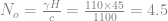
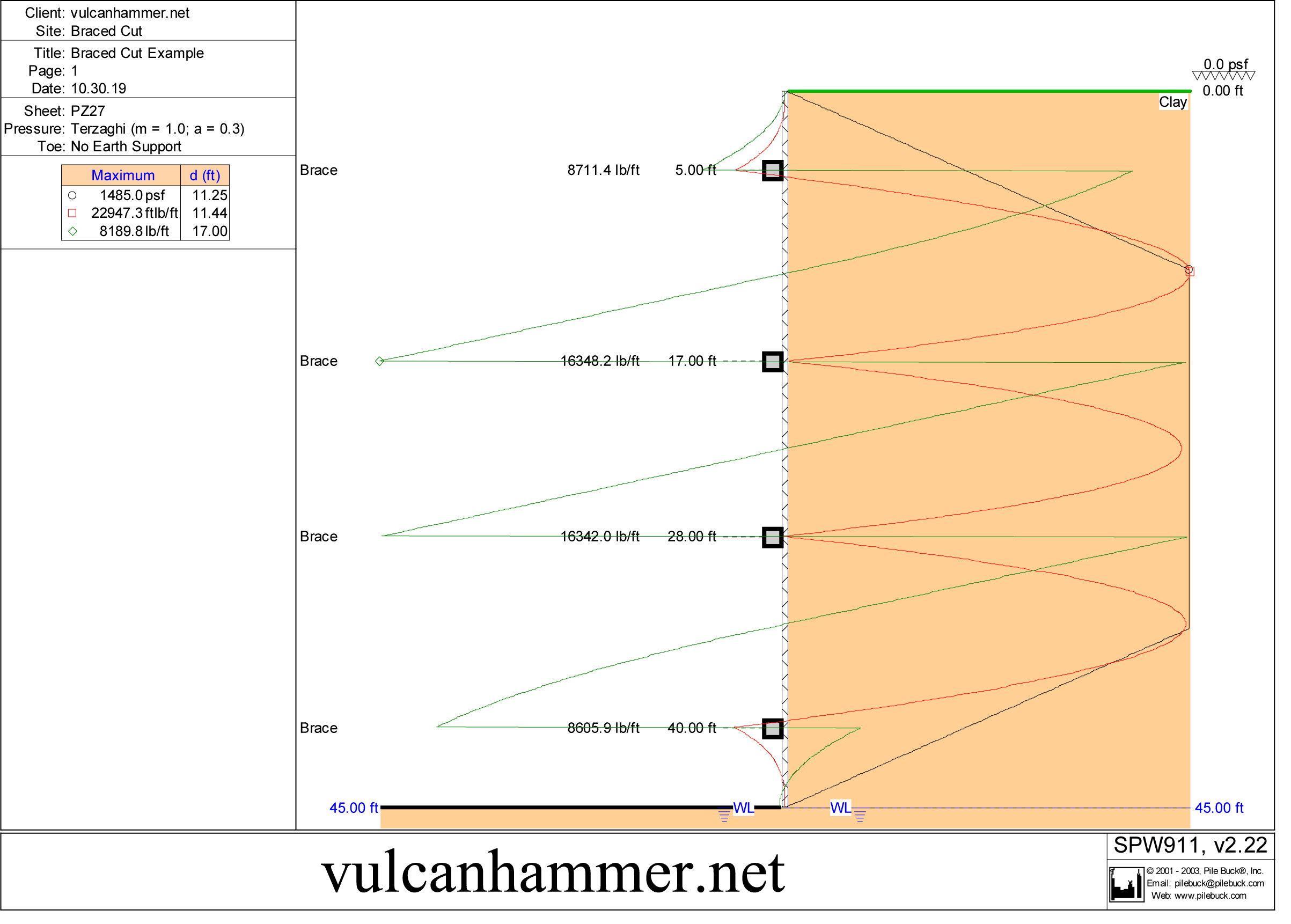
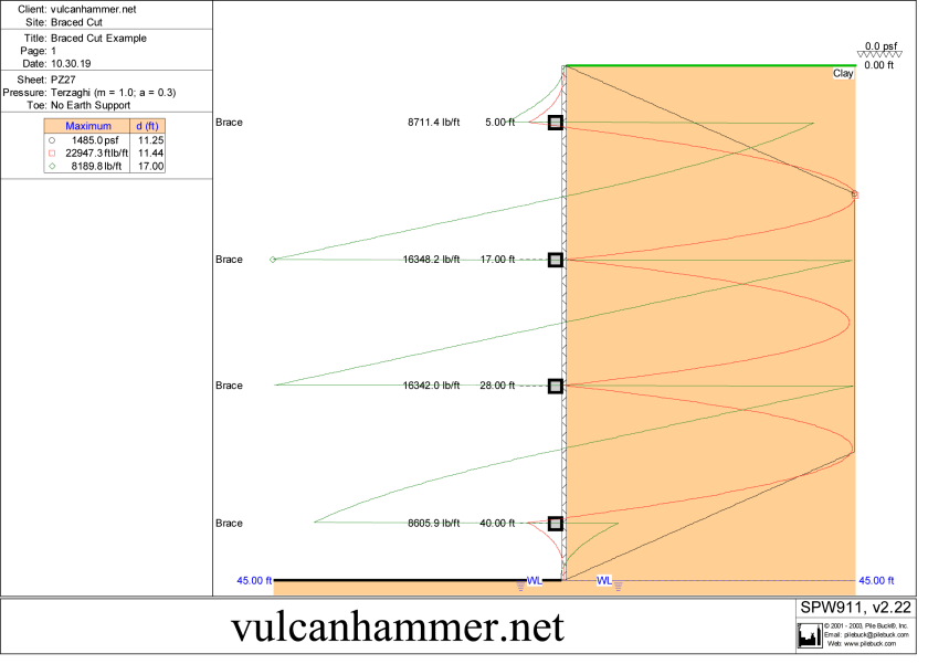
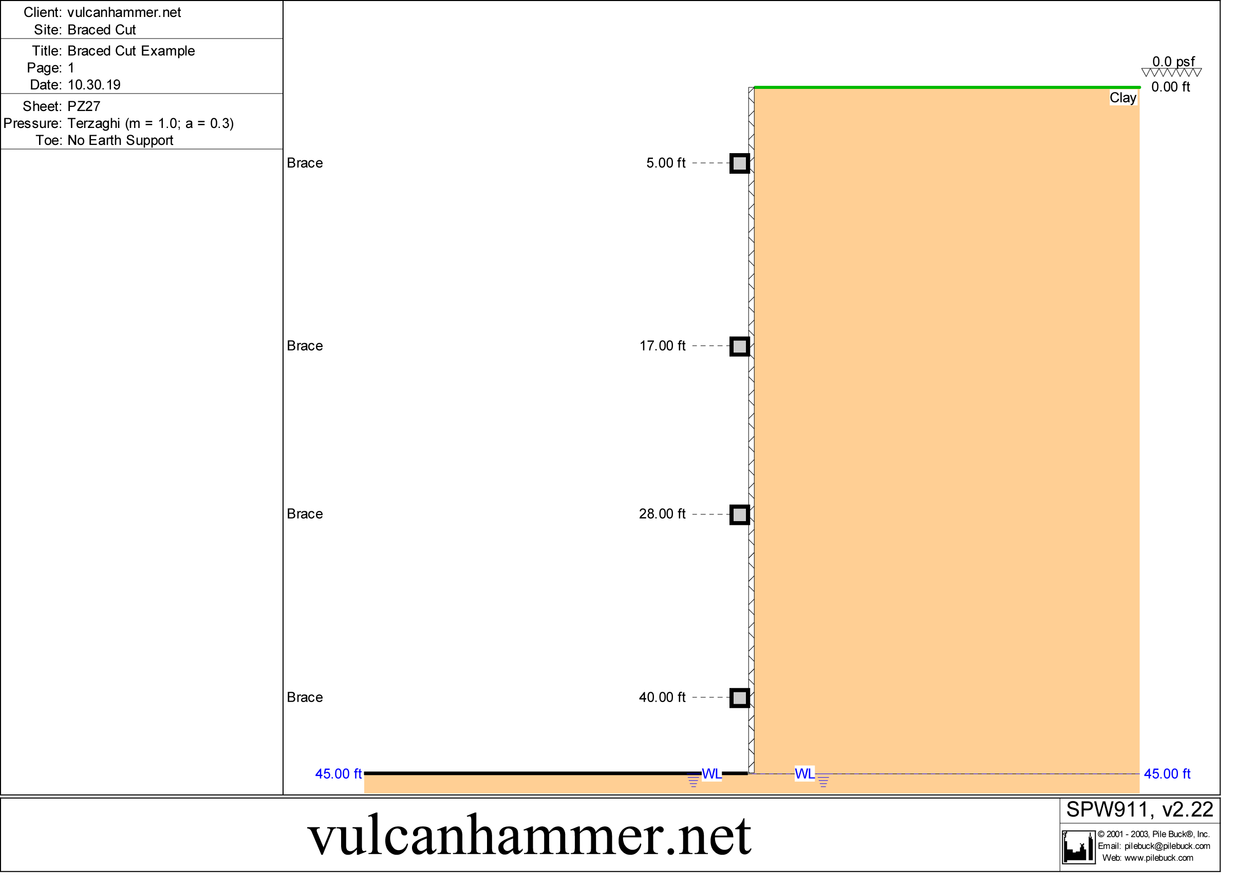
Let us consider a braced cut excavation which is 45′ deep and which has supports at a depth of 5′, 17′, 28′ and 40′. The soil behind the wall is uniform with c = 1100 psf and γ = 110 pcf. The water table is at the bottom of the excavation and does not enter into our calculations. To show how this lays out we’ll use Pile Buck’s SPW 911 sheet pile software. We’ll assume PZ-27 sheeting is being used, and that there is no surcharge on the wall.
Basic layout of braced cut example, using Pile Buck’s SPW-911 software
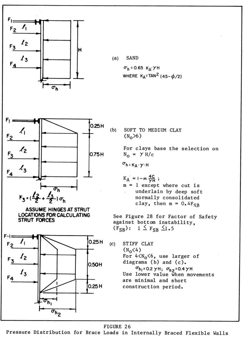
We obviously have a clay soil, thus our selection will be either (b) or (c). Whether the soil is soft to medium or stiff depends upon the stability number , which is computed as follows:
This is between (b) and (c), we are thus supposed to use the “larger” of the two diagrams. The earth pressure coefficient for (b) is
Assuming m = 1,
and thus
If we turn to Case (c) and assume that
this is obviously “larger” than Case (b), so we will use Case (c), even when using a “medium” case between the two extreme pressure profiles.
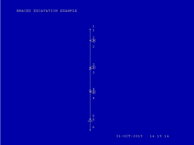
We thus have a pressure distribution that can be described as follows:
Beginning at the top, it linearly rises from zero to the maximum value of 1485 psf at a point a quarter down the wall, or 45/4 = 11.25′.
From that point until a quarter from the bottom of the wall, or 0.75 * 45 = 33.75′, it is a constant pressure of 1485 psf.
From that point until the bottom of the wall, it linearly decreases to a value of zero at the bottom of the wall.
We will analyse the wall using two different approaches to the structural analysis and three different implementations:
Hinged Solution
CFRAME finite element software
SPW 911 sheet pile software
Continuous Solution: CFRAME finite element software
Turning to the structural aspects of the wall, the guidelines for dividing the wall up for the hinged method are as follows:
If the wall is cantilevered at either end, then the endmost support and the one next to it form a simply supported beam with a cantilever at one end and a distributed load.
Segments in the middle are analysed as simply supported beams with a distributed load.
If there’s a support at the top or the bottom of the wall, the beam at that location is analyzed as a simply supported beam.
Reactions are computed for each beam. For supports where two segments meet, you simply add the two reactions from each beam for a total reaction for the support.
Maximum moments are computed for each beam; the largest of these maximum moments is the maximum moment of the system and the one used to size the sheeting.
Since the distributions are simple, “handbook” type formulas can be used. The trout in the milk takes place (as it does here) when the break points in the distribution don’t coincide with the supports, in which case you end up with a more complicated distribution. There are two ways of dealing with this problem.
The first is to reduce the distributed loads to point load resultants. This is a favourite tactic among geotechnical engineers and is used extensively with shallow foundations. For purely hand calculations, it makes sense. The moments will be higher (which is conservative) but the reactions will be identical, assuming the concentration of the moments went off according to plan.
The second is to employ beam software to analyse each segment. Although there’s a lot of beam software out there, being the old coots we are, we’ll use CFRAME, a DOS program for two-dimensional structures. It gets the job done and is fairly easy to use. (Note: because of some bad interaction between CFRAME and DOSBox, we ran it on a Windows XP installation. The manual for CFRAME: Computer Program with Interactive Graphics of Plane Frame Structures is here.)
We will also use the SPW 911 software to compare the results, which also uses the hinged method of structural analysis.
Implementation in CFRAME
The first thing we need to do is to specify the distributed loads. CFRAME, like most finite element programs, considers the beam between each support (and the beams from the outermost supports to the cantilever element) as one element. So there are six elements. CFRAME asks us to specify the distributed load (constant or linearly varying) for each element, and requires us to specify the constant loads and the varying loads separately.
But here we run into something that trips up students. Sheet piles are analysed as beams, but they’re “infinite” beams; we analyse them in terms of moment of inertia per length of wall, section modulus per length of wall, load per unit length of wall, etc. The good news is that, for distributed loads, the pressure at any point is the load per unit length! Pressure is expressed, in this case, as lb/ft^2 of wall, when in reality it’s lb/ft/ft of wall. That makes things simpler; as long as we enter the moment of inertia and cross sectional area in terms of “per foot of wall” (which any US unit section should furnish us) then we’re good. In this case for PZ-27 the moment of inertia is 184.2 in^4/ft of wall and the cross-sectional area is 7.94 in^2/ft of wall, and these are entered directly into CFRAME.
With that technicality out of the way, for are areas of constant earth pressure (the middle) we’re also good; it’s just 1485 psf, and we enter this directly into CFRAME. With the ramped portions, they increase from the top and bottom of the wall at a rate of 1485/11.25 = 132 psf/ft from the end. Looking at the topmost element, which we enter into CFRAME as (surprise!) element 1, the pressure at the topmost support is 132 * 5 = 660 psf, which we enter as the maximum pressure for the “triangle load” on the top element.
For element 2, we have two loads. The first is a continuation of the ramped load from 660 psf at the top end of the beam to 1485 psf at a point 11.25′ from the top of the wall or 11.25′ – 5′ = 6.25′ from the top end of the beam. The second load is simply a constant load to the bottom end of the beam.
The middle element 3 has a constant distribution across its entire length. The bottom two elements are mirror images of the top two elements.
Results from CFRAME
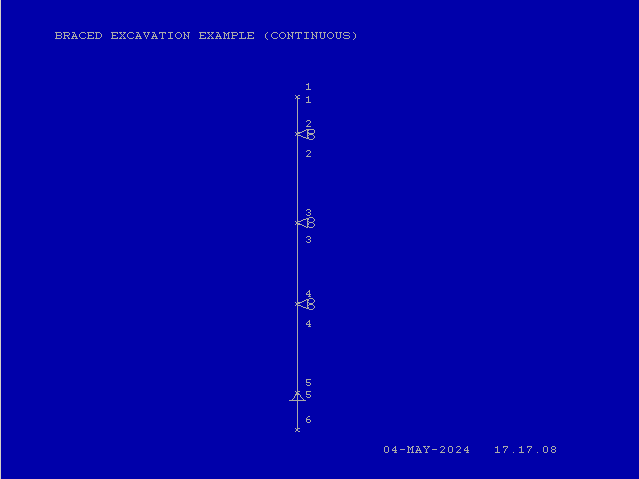
We entered the data into CFRAME via a small text file. First we present the model itself.
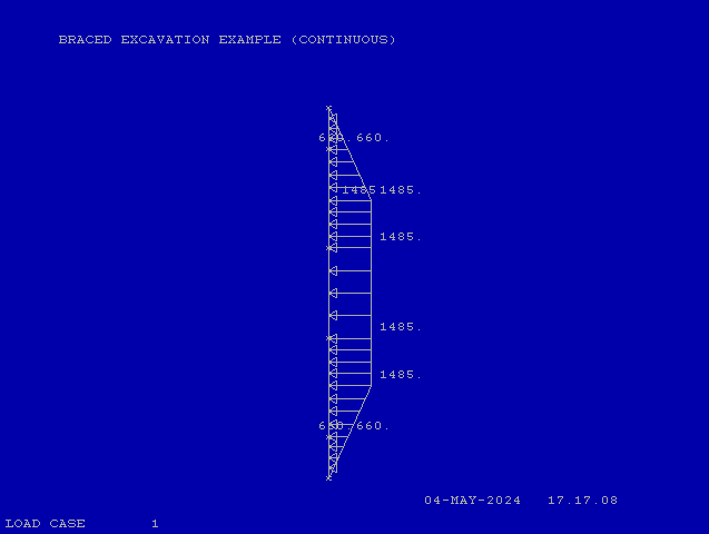
The basic layout of the model. The model is simply supported at all braces. Additionally–and this is one reason we wanted to use CFRAME–the central element 3 was additionally pinned at the ends to simulate Terzaghi and Peck’s original intent for the method.The pressure distribution on the model, replicating that Terzaghi and Peck distribution for stiff clays.
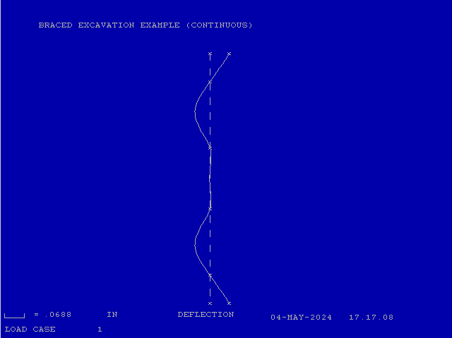
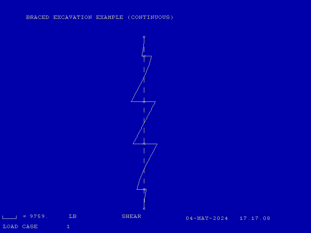
Now we show the results.
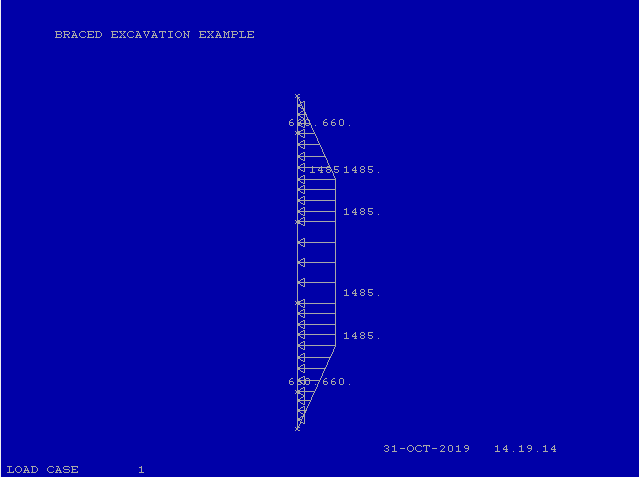
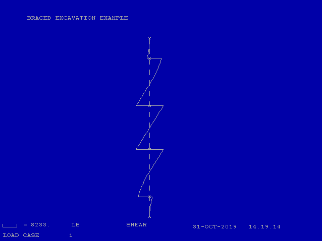
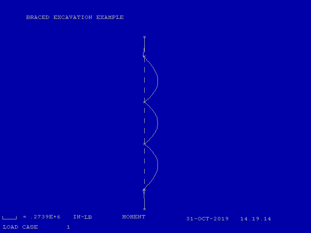
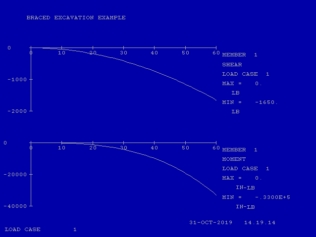
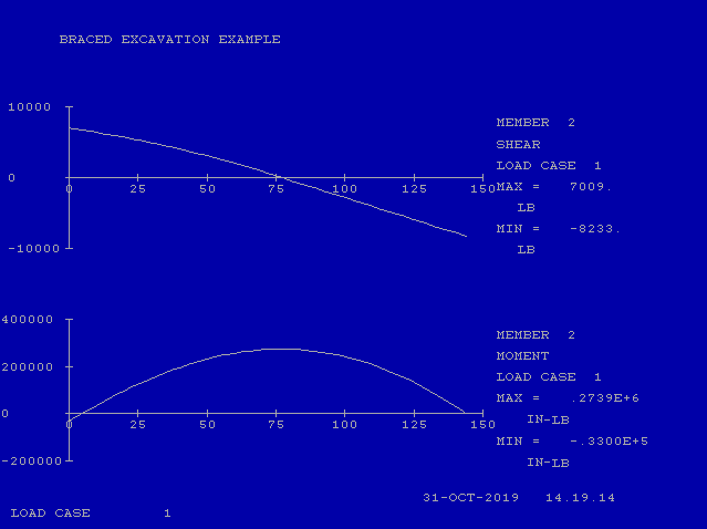
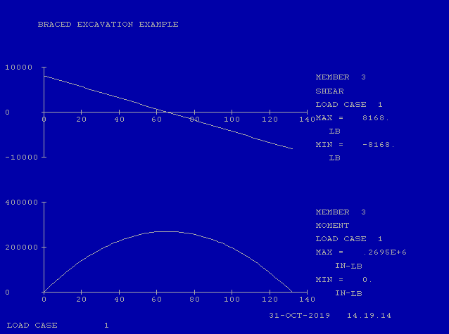
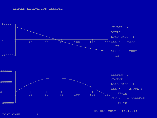
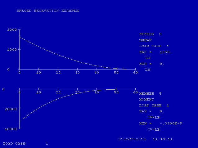
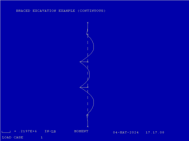
The deflections of the model. The pinned (discontinuous) nature of the middle element 3 can be easily seen.The shear diagram for the model. As is the case for all of these diagrams, the maximum value can be seen in the lower left corner of the image.The moment diagram for the braced excavation. Although it is not explicit, the values for shear and moment are per foot of wall. As with the deflection, the effects of pinning the ends of element 3 are easily seen.
First let’s look at the reactions at the supports, which come from the element results. They are as follows:
Support 1 (Node 2): The reaction/shear at that point from element 1 is 1650 lb/ft of wall and from element 2 7009 lb/ft of wall, summing it comes to 8659 lb/ft of wall.
Support 2 (Node 3): The reaction/shear at that point from element 2 is 8233 lb/ft and from element 3 8168 lb/ft, summing it comes to 16401 lb/ft.
Support 3 (Node 4) is the same as Node 3 by symmetry.
Support 4 (Node 5) is the same as Node 2 by symmetry.
Thus the maximum brace load is on Supports 2 and 3, 16401 lb/ft. We have for convenience ignored the sign conventions and simply added the reactions, since they’re all in the same direction.
The maximum moment is actually in Element 2 (or 4,) and is 273,900 in-lb/ft of wall. Since the elastic section modulus for PZ-27 is 30.2 in^3/ft of wall, the maximum bending stress is 273,900/30.2 = 9070 psi, which is well within most allowable specifications. A lighter section can probably be employed, depending upon the allowable deflection and other requirements.
As a quick check, for a uniformly distributed load on a simply supported beam, the maximum moment is given by the equation
Substituting the values for Element 3, we have
Analysis with SPW 911
Now we compare these with SPW 911, whose output is as follows:
The results are compared with each other below.
Solution II: Continuous Solution
The setup for this solution, except for the beam itself, is very similar to the hinged solution. First, the basic structural model is shown.
Structural Model for the braced excavation example. Note that the only difference between this model and the hinged model is that the hinges at nodes 3 and 4 have been removed. CFRAME is advantageous for this type of analysis in that it uses “classical” models of fixity at the nodes. thus the “massaging” of this fixity in some FEA code is eliminated.Pressure distribution on the sheet pile walls, which is identical to the hinged method.Deflection results. These are very different from the hinged method. One thing that is not included in the CFRAME model is the deflection of the brace/strut nodes themselves, which was an important consideration in Terzaghi and Peck’s development of this method (although it doesn’t appear in the hinged method either.)Shear diagram with the continuous beam.Moment diagram for the continuous beam.
The simplest way of comparing all three methods is to tabulate the highlights. Let us begin by looking at the brace/strut loads.
Strut Loads, lb/ft of wall
Analysis Method
Node 2/ Strut 1
Node 3/ Strut 2
Node 4/ Strut 3
Node 5/ Strut 4
CFRAME, Hinged Method
8659
16400
16400
8659
SPW 911
8711
16348
16342
8606
CFRAME, Continuous Method
7133
17930
17930
7133
Comparison of Brace/Strut Loads for Different Methods
As one would expect, the CFRAME hinged method and SPW 911 are very close, as both hinge the beams. The continuous method tends to shift the loading to the vertical centre of the wall; the brace loads are less at the top and the bottom and greater at the centre. If the braces, for example, are designed for the maximum strut load, they would be sized larger using the continuous method.
Now we look at the maximum shears and moments.
Maxima
Analysis Method
Shear, lb/ft
Moment, ft-lb/ft
CFRAME, Hinged Method
8233
22825
SPW 911
8199
22947
CFRAME, Continuous Method
9759
18308
Comparison of Maximum Shear and Moments for Different Methods
As was the case with the brace/strut loads, CFRAME hinged method and SPW 911 are very close. The continuous method has a higher maximum shear load but a lower maximum moment, which means that using the continuous method would probably result in using lighter sheeting.
The steel sheet piling may be designed either as a continuous beam supported at the strut levels or by assuming pins exist at each strut thereby making each span statically determinant. It is also customary to assume a support at the bottom of the excavation.
In terms of raw conservatism, the two methods (hinged and continuous) are different. The hinged method resulted in a lower maximum strut load but the continuous method resulted in a lower sheeting moment. This may not hold for all cases; the relationship between the two may vary with differences in the number and spacing of struts and different soil loading profiles.
You might not think that geotechnical engineering would have anything to do with the Apollo 11 mission that put the first humans on the surface of the moon, but you would be wrong. The landing pads of the lunar excursion module (LEM) had to act as footings on the surface of the moon. If they […]


 is the uniform pressure on the foundation in load per unit area, and
  is the width of the foundation, usually expressed in American practice as
  . The angles are as shown. The stresses are as follows:
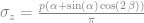


 , any point in the half space can be defined. They can be related to the Cartesian coordinates as follows:

 and
and  , which means that the soil stress is equal to the foundation pressure
![K_z=\frac{2}{\pi}\left[arctan\left(\frac{b}{2z}\right)+\frac{bz}{\frac{b^2}{2}+2z^{2}}\right],\,y=0](https://s0.wp.com/latex.php?latex=K_z%3D%5Cfrac%7B2%7D%7B%5Cpi%7D%5Cleft%5Barctan%5Cleft%28%5Cfrac%7Bb%7D%7B2z%7D%5Cright%29%2B%5Cfrac%7Bbz%7D%7B%5Cfrac%7Bb%5E2%7D%7B2%7D%2B2z%5E%7B2%7D%7D%5Cright%5D%2C%5C%2Cy%3D0+&bg=ffffff&fg=777777&s=0&c=20201002)
 and
and  , the tabulation of these coefficients is shown below.
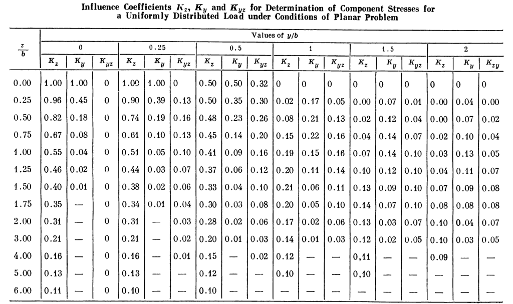
 , not necessarily to the centre of the foundation.
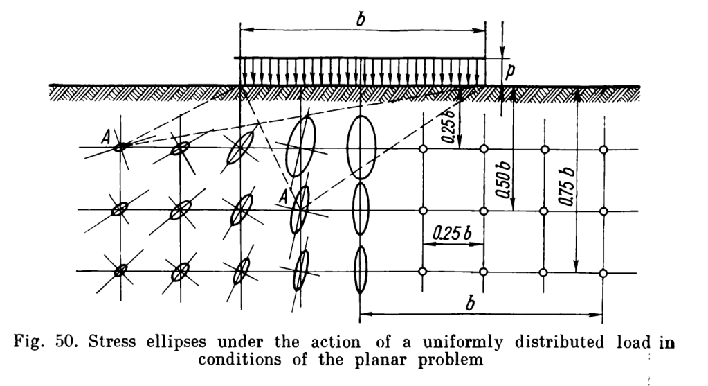


 (the influence coefficient for the vertical stresses)
 (the aspect ratio of the foundation or the part of the foundation of its length (longer side) divided by its width (shorter side)
 the aspect ratio of the foundation or part of the foundation of the depth from the corner to its shorter side.
 :
:
 :
:


 . The values for
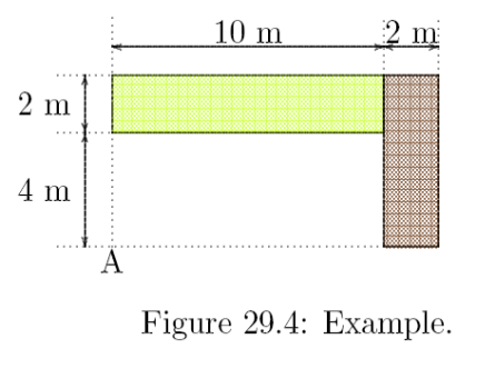


 settlement of the foundation at the point of interest
 influence factor, given in the table below
 uniform pressure on the foundation
 smaller dimension of rectangle or dimension of square side
 Poisson’s Ratio of the soil
 Modulus of elasticity of the soil
 are given below, both for a soil layer of large depth and one of limited depth
  .
.


 , which is computed as follows: