It is with sadness that we report the death of Dr. Harry M. Coyle, professor of civil engineering at Texas A&M University from 1964 to 1987, back in January. You can read the entire obituary here.
For those of us involved in deep foundations, his name is a familiar one, and his monographs have graced this site and its companion, vulcanhammer.info, for many years. Among other things he is known for the Coyle and Castello method for estimating pile capacity in sand, the Coyle and Gibson method for determining damping for pile dynamics analysis, and the co-developer of the PX4C3 routine for axial load-settlement estimation, which we feature on this site, and which is the ancestor of many of those in use today. He was deeply involved in the development of the TTI wave equation program, and some of his work relating to that is here.
Our continued condolences and prayers go to his family, and, as the obituary states, “Having loved his friends and family well, Harry Coyle will be missed by all until we are reunited with him in Glory. “
Recently I had a round of correspondence with a county official in Washington state re pile drivability studies and their place in the contract process. (If you’re looking for some explanation of this, you can find it here). His question was as follows:
During the bidding process, is the contractor’s sole basis for anticipating the size of the hammer needed the WEAP analysis? Does a contractor rely solely on design pile capacities or does the contractor combine geotechnical boring logs and cross-sections with his expertise? Who will be ultimately responsible that a large enough hammer is considered in the bid and brought to the site, the contractor or the preparer of the design package?
My response was as follows:
First, at this time the WEAP analysis is the best way for contractor and owner alike to determine the size of a hammer (both to make sure it isn’t too small with premature refusal, or too large and excessive pile stresses) necessary to install a certain pile into a certain soil.
It is a common specification requirement for a contractor to furnish a wave equation analysis showing that a given hammer can drive a pile into a given soil profile. As far as what soil profile is used, that’s a sticky issue in drivability studies. Personally I always attempt to estimate the ultimate axial pile capacity in preparation of a wave equation analysis. There are two important issues here.
The first is whether the piles are to be driven to a “tip elevation” specification vs. a blow count specification. For the former, an independent pile capacity determination is an absolute must. For the latter, one might be able to use the pile capacities if and only if he or she can successfully “back them out” from the allowable capacities, because the design factors/factors of safety will vary from one job and owner to the next. Some job specs make that easy, most don’t.
Even if this can be accomplished, there is the second problem: the ultimate capacity of interest to the designer and the one of interest to the pile driver are two different things. Consider this: the designer wants to know the pile with the lowest capacity/greatest settlement for a given load. The pile driver wants to know the pile with the highest capacity. If you use the design values, you may find yourself unable to drive many of the piles on a job or only with great difficulty. I’m seeing a disturbing trend towards using the ultimate capacity for design and running into drivability problems.
As far as responsibility is concerned, that of course depends upon the structure of the contract documents. I’ve discussed the contractor’s role; I would like to think that any driven pile design would include some consideration of the drivability of the piles.
Some of the FHWA publications I offer both in print and online (including the Driven Pile Manual) have sample specifications which you may find helpful.
Hope this long diatribe is of assistance.
After this, there’s another way of looking at this problem from an LRFD (load and resistance factor design) standpoint that might further illuminate the problem. The standard LRFD equation looks like this:
This is fine for design. With drivability, however, the situation is different; what you want to do is to induce failure and move the pile relative to the soil with each blow. So perhaps for drivability the equation should be written as follows:
It’s worthy of note that, for AASHTO LRFD (Bridge Design Specifications, 5th Edition) can run from 0.9 to 1.15, which would in turn force the load applied by the pile hammer upward more than it would if typical design factors are used. Given the complexity of the loading induced by a hammer during driving, the LRFD equation is generally not employed directly for drivability studies, and the fact that hovers around unity makes the procedure in LRFD very similar to previous practice.
The problem I posed re the hardest pile to drive vs. the lowest capacity pile on the job is still valid, especially with non-transportation type of projects where many piles are driven to support a structure. When establishing a “standard” pile for capacity, it is still the propensity of the designer to select the lowest expected pile capacity of all the pile/soil profile combinations as opposed to the highest expect pile resistance of all the pile/soil profile combinations necessary for drivability studies.
Put another way, the designer will tend to push the centre of the probability curve lower while the pile driver will tend to push the centre of the probability curve higher. This is a design process issue not entirely addressed by LRFD, although LRFD can be used to help explain the process.
This is the first installment of a new series on the development of the STADYN wave equation program for analyzing impact driven foundation piles. This program was the subject of this study and what you’ll see on this site is the sequel to that study.
The first in the series, however, isn’t really about technical aspects of the program and application, but something more mundane: formatting the output in a way that one can easily read the output. Although STADYN is written in FOTRAN 77 (with extensions) the techniques shown here are useful elsewhere and in other languages. In fact, techniques similar to these were used in the development of this routine, which is in PHP.
Engineers have done tabular output in regimented text format for many years. While it gets the job done, it’s not very pretty or easy to read, and requires some very regimented formatting to keep the columns straight. The simplest way to illustrate this is to use a worked example. Although ultimately the idea is to apply this to STADYN, the program used is a revision of the BENT1 program which is available on this site and goes back to the 1970’s.
BENT1 is a program designed to analyze pile groups for axial and lateral response to loading, and is in fact the ancestor of programs such as the COM624 series (it’s the first of those,) LPILE and APILE. It starts off with output that looks like this:
EX 1  COPANO BAY CAUSEWAY, ARKANSAS COUNTY TEXAS, US HIGHWAY 35


          LIST OF INPUT DATA ---


          PV              PH             TM           TOL    KNPL KOSC
     0.8440E+06     0.3640E+05     0.1682E+08     0.1000E-02  4    0


        CONTROL DATA FOR PILES AT EACH LOCATION

     PILE NO    DISTA        DISTB      BATTER         POTT       KS   KA
         1    -0.1260E+03  0.0000E+00 -0.2440E+00  0.1000E+01    1   1
         2    -0.9000E+02  0.0000E+00  0.0000E+00  0.2000E+01    1   1
         3     0.9000E+02  0.0000E+00  0.0000E+00  0.2000E+01    1   1
         4     0.1260E+03  0.0000E+00  0.2440E+00  0.1000E+01    1   1


  PILE NO.  NN         HH            DPS      NDEI   CONNECTION FDBET
     1     31    0.36000E+02    0.12000E+03    1      FIX    0.0000E+00
     2     31    0.36000E+02    0.12000E+03    1      FIX    0.0000E+00
     3     31    0.36000E+02    0.12000E+03    1      FIX    0.0000E+00
     4     31    0.36000E+02    0.12000E+03    1      FIX    0.0000E+00
Note the text is all caps (typical for the era) and formatted in a fixed-pitch format. The programmer had to exercise some care to get the columns and headers lined up properly, which in FORTRAN 77 could be a job.
HTML documents—which are still, in their various forms, what you see most often when you browse the web—are basically ASCII text documents with formatting markup. This is also true of XML documents as well. Just about any language can readily generate ASCII files, and FORTRAN 77 is no exception. One of the biggest changes in the Internet, however, is that, in the early days, HTML documents were generated by hand (including the markup) and were uploaded to a server as static web pages. Today virtually all pages are generated « dynamically » to varying degrees. (The major downside to dynamic generation is that many security flaws in web pages come from holes in the code, but that’s another post.) In a sense we’re going to make FORTRAN 77 become a dynamic page generator.
Getting back to the output above, the first line was generated by the following code:
Here the title is read one character at a time into a character array, converted to upper case using the « UPPER » routine, and then output to the file using the same format statement it was read with.
Turning to how to do this in HTML—and the HTML you’re going to see here is very old and basic—we start by generating the header for the page with this code:
 write(4,*)'<head><title>BENT2 Run for Case ',casenm,
&'</title></head><body>
<div align="center">'
Just about all HTML pages have a header, and here we use the case name variable to « personalise » the title, which appears at the top of the page. Note also that, when we transition to the body portion of the page, we use a div tag to center all of the content. That’s a matter of personal preference. It’s also possible to put CSS in the head as well, which opens up possibilities to liven up the page. Whether you do that depends upon how deep into HTML you want to get. With twenty years of experience doing this, I could have done more, but what you’ll see will be an improvement.
From here we change the last line of the original code shown above to generate the title as follows:
The header tags (Level 2, I think Level 1 generally makes it too large) are placed at the start and end of line and the title is in the middle. We could have gotten rid of the all-caps business, but for starters we did not.
Now to the tabular data. The title and table immediately below the original code was generated using this:
     WRITE(4, 150)
 150 FORMAT ( // , 5X, ' LIST OF INPUT DATA ---'
    & /// 4X, ' PV PH '
    & , ' TM TOL KNPL KOSC')
     WRITE(4, 160) PV, PH, TM, TOL, KNPL, KOSC
 160 FORMAT (4E15.4, I3, I5)
This is a simple one-row table with a header above it. Doing this in HTML using HTML tables (which, I know, are hopelessly obsolete but in this case handy) results in the following:
 WRITE (4,110)
110 FORMAT ('
<table border="2" cellspacing="2" cellpadding="3">',
&'<caption>List of Input Data</caption>',
&'
<tr>
<td>Vertical Load on Foundation, kips</td>
',
&'
<td align="center">Horizontal Load on Foundation, kips</td>
',
&'
<td align="center">Moment on Foundation, in-kips',
&'</td>
<td align="center">Iteration Tolerance, in.',
&'</td>
<td align="center">Number of Pile Locations',
&'</td>
<td align="center">Solution Oscillation Control</td>
</tr>
')
WRITE (4,120) 0.001*pv,0.001*ph,0.001*tm,tol,knpl,kosc
120 FORMAT ('
<tr>
<td>',4(g15.4,'</td>
<td align="center">'),
&i3,'</td>
<td align="center">',i5,
&'</td>
</tr>
</table>
')
The last table shown earlier is only slightly harder to write. The original code (which includes the read statement) is as follows:
      WRITE(4, 170)
  170 FORMAT ( // , 5X, '   CONTROL DATA FOR PILES'
     &     , ' AT EACH LOCATION ' // 4X, ' PILE NO   '
     &     , ' DISTA        DISTB      BATTER         '
     &     , 'POTT       KS   KA')
      DO 200 K = 1, KNPL
      READ(3,*) LINNO, DISTA(K), DISTB(K), THETA(K),
     &      POTT(K), KS(K), KA(K)
      WRITE(4, 190)   K, DISTA(K), DISTB(K),
     &      THETA(K), POTT(K), KS(K), KA(K)
  180 FORMAT (4E10.4, 2I5)
  190 FORMAT (5X, I5, 1E15.4, 3E12.4, I5, I4)
  200 CONTINUE
The biggest difference is the need to write multiple table rows. On the other hand, we were able to combine two tables into one, which makes for easier reading.
Note: WordPress (which powers this site) may power a quarter of the web, but it’s a very “vertical” format and doesn’t always “do horizontal” very well. With non-mobile devices, the wider tables will bleed off to the right, but you can see them. With mobile devices, it just cuts them off because these don’t have a left-right scroll. Also, it doesn’t always reproduce FORTRAN 77 code very gracefully, we apologize for the inconvenience.
The final result of all of this coding looks like this:
EX 1 COPANO BAY CAUSEWAY, ARKANSAS COUNTY TEXAS, US HIGHWAY 35
List of Input Data
Vertical Load on Foundation, kips
Horizontal Load on Foundation, kips
Moment on Foundation, in-kips
Iteration Tolerance, in.
Number of Pile Locations
Solution Oscillation Control
844.0
36.40
0.1682E+05
0.1000E-02
4
0
Control Data for Piles at Each Location
Pile Number
Horizontal Coordinate of Pile Top, in.
Vertical Coordinate of Pile Top, in.
Batter, Degrees
Number of Piles at Location
p-y Curve Identifier
t-z Curve Idenfifier
Number of Pile Increments
Increment Length, in.
Distance from Pile Head to Soil Surface, in.
Number of Flexural Stiffness Values
Head Connection of Pile
Rotational Restraint Value
1
-126.0
0.0000
-13.98
1.000
1
1
31
36.000
120.00
1
FIX
0.0000
2
-90.00
0.0000
0.0000
2.000
1
1
31
36.000
120.00
1
FIX
0.0000
3
90.00
0.0000
0.0000
2.000
1
1
31
36.000
120.00
1
FIX
0.0000
4
126.0
0.0000
13.98
1.000
1
1
31
36.000
120.00
1
FIX
0.0000
So how does this look when implemented in STADYN? We’ll start with the case which compares STADYN’s output with Finno (1989,) and the output (after complete conversion to HTML) looks like this:
Output for STADYN Wave Equation Program
Case finno2, 7: 5:41:78 9 May 2017
Hammer Properties
Ram Mass, kg
0.295E+04
Hammer Equivalent Stroke, mm
914.
Hammer Efficiency, Percent
67.0
Ram Velocity at Impact, m/sec
3.46
Ram O.D., mm
286.
Ram I.D., mm
0.000
Cross-Sectional Area of Ram, mm**2
0.642E+05
Ram Length, mm
0.583E+04
Cap Properties
Mass of Cap, kg
465.
Cap O.D., mm
483.
Cap I.D., mm
0.000
Cap Body Thickness, mm
323.
Cushion Thickness, mm
127.
Cushion Material
Micarta & Aluminium
Cushion Area Same as Ram
Pile Properties
Pile Length, m
15.5
Pile Length Immersed in Soil, m
15.2
Head Cross-Sectional Area, mm**2
0.134E+05
Head Impedance, kN-sec/m
541.
omega2 (c/L), 1/sec
330.
2L/c,msec
6.07
Number of Complete Cycles for Pile Stress Wave, L/c
8
Ratio of Actual to Ideal Interface Stiffness
4.00
Minimum Distance from Pile for Model Side, m
15.0
Width of Soil Box (x), m
15.2
Depth of Soil Box (y), m
30.5
Material Properties for Hammer and Pile Materials
Material Type
Material Code
Modulus of Elasticity, MP
Poissons Ratio
Density, kg/m^3
Cohesion, MPa
Yield Strength MPa
Phi Degrees
Psi Degrees
Acoustic speed, m/sec
Steel
1
0.207E+06
0.300
0.788E+04
0.131E+04
0.262E+04
0.000
0.000
0.512E+04
Concrete
2
0.275E+05
0.300
0.241E+04
50.0
100.
0.000
0.000
0.338E+04
Wood
3
0.965E+04
0.300
800.
75.0
150.
0.000
0.000
0.347E+04
Aluminium
4
0.690E+05
0.300
0.271E+04
0.100E+04
0.200E+04
0.000
0.000
0.504E+04
Micarta & Aluminium
5
0.241E+04
0.300
0.183E+04
100.
200.
0.000
0.000
0.115E+04
Data for Region 1 (Pile )
Number of Nodes in a Regional Row
2
Number of Full Element Columns
1
Geometric Squeeze in x-direction
1
Number of Nodes in a Regional Column
2
Number of Full Element Rows
1
Geometric Squeeze in y-direction
1
Region Material
Steel
2(x = 219.1, y = -304.8), mm
10
3(x= 228.6, y= -304.8), mm
100
Corner Locations Nodes and Connectivity
100
1(x = 219.1, y = 0.0), mm
2
4(x = 228.6, y = 0.0), mm
Data for Region 2 (Pile )
Number of Nodes in a Regional Row
2
Number of Full Element Columns
1
Geometric Squeeze in x-direction
1
Number of Nodes in a Regional Column
16
Number of Full Element Rows
1
Geometric Squeeze in y-direction
1
Region Material
Steel
2(x = 219.1, y = 0.0), mm
1
3(x= 228.6, y= 0.0), mm
100
Corner Locations Nodes and Connectivity
5
1(x = 219.1, y = 15211.4), mm
3
4(x = 228.6, y = 15211.4), mm
Data for Region 3 (Pile )
Number of Nodes in a Regional Row
2
Number of Full Element Columns
1
Geometric Squeeze in x-direction
1
Number of Nodes in a Regional Column
2
Number of Full Element Rows
1
Geometric Squeeze in y-direction
1
Region Material
Steel
2(x = 219.1, y = 15211.4), mm
2
3(x= 228.6, y= 15211.4), mm
100
Corner Locations Nodes and Connectivity
6
1(x = 0.0, y = 15220.9), mm
4
4(x = 228.6, y = 15220.9), mm
Data for Region 4 (Pile )
Number of Nodes in a Regional Row
2
Number of Full Element Columns
1
Geometric Squeeze in x-direction
1
Number of Nodes in a Regional Column
2
Number of Full Element Rows
1
Geometric Squeeze in y-direction
1
Region Material
Steel
2(x = 0.0, y = 15220.9), mm
3
3(x= 228.6, y= 15220.9), mm
100
Corner Locations Nodes and Connectivity
7
1(x = 0.0, y = 15240.0), mm
8
4(x = 228.6, y = 15240.0), mm
Data for Region 5 (Soil )
Number of Nodes in a Regional Row
21
Number of Full Element Columns
20
Geometric Squeeze in x-direction
3
Number of Nodes in a Regional Column
16
Number of Full Element Rows
3
Geometric Squeeze in y-direction
1
2(x = 228.6, y = 0.0), mm
100
3(x= 15240.0, y= 0.0), mm
2
Corner Locations Nodes and Connectivity
101
1(x = 228.6, y = 15211.4), mm
6
4(x = 15240.0, y = 15211.4), mm
Data for Region 6 (Soil )
Number of Nodes in a Regional Row
21
Number of Full Element Columns
20
Geometric Squeeze in x-direction
3
Number of Nodes in a Regional Column
2
Number of Full Element Rows
3
Geometric Squeeze in y-direction
1
2(x = 228.6, y = 15211.4), mm
5
3(x= 15240.0, y= 15211.4), mm
3
Corner Locations Nodes and Connectivity
101
1(x = 228.6, y = 15220.9), mm
7
4(x = 15240.0, y = 15220.9), mm
Data for Region 7 (Soil )
Number of Nodes in a Regional Row
21
Number of Full Element Columns
20
Geometric Squeeze in x-direction
3
Number of Nodes in a Regional Column
2
Number of Full Element Rows
3
Geometric Squeeze in y-direction
1
2(x = 228.6, y = 15220.9), mm
6
3(x= 15240.0, y= 15220.9), mm
4
Corner Locations Nodes and Connectivity
101
1(x = 228.6, y = 15240.0), mm
9
4(x = 15240.0, y = 15240.0), mm
Data for Region 8 (Soil )
Number of Nodes in a Regional Row
2
Number of Full Element Columns
1
Geometric Squeeze in x-direction
1
Number of Nodes in a Regional Column
21
Number of Full Element Rows
1
Geometric Squeeze in y-direction
3
2(x = 0.0, y = 15240.0), mm
4
3(x= 228.6, y= 15240.0), mm
100
Corner Locations Nodes and Connectivity
9
1(x = 0.0, y = 30480.0), mm
101
4(x = 228.6, y = 30480.0), mm
Data for Region 9 (Soil )
Number of Nodes in a Regional Row
21
Number of Full Element Columns
20
Geometric Squeeze in x-direction
3
Number of Nodes in a Regional Column
21
Number of Full Element Rows
3
Geometric Squeeze in y-direction
3
2(x = 228.6, y = 15240.0), mm
7
3(x= 15240.0, y= 15240.0), mm
8
Corner Locations Nodes and Connectivity
101
1(x = 228.6, y = 30480.0), mm
101
4(x = 15240.0, y = 30480.0), mm
Data for Region 10 (Hammer )
Number of Nodes in a Regional Row
2
Number of Full Element Columns
1
Geometric Squeeze in x-direction
1
Number of Nodes in a Regional Column
2
Number of Full Element Rows
1
Geometric Squeeze in y-direction
1
Region Material
Steel
2(x = 219.1, y = -304.8), mm
11
3(x= 228.6, y= -304.8), mm
100
Corner Locations Nodes and Connectivity
100
1(x = 219.1, y = -304.8), mm
1
4(x = 228.6, y = -304.8), mm
Data for Region 11 (Hammer )
Number of Nodes in a Regional Row
2
Number of Full Element Columns
1
Geometric Squeeze in x-direction
1
Number of Nodes in a Regional Column
2
Number of Full Element Rows
1
Geometric Squeeze in y-direction
1
Region Material
Steel
2(x = 14.3, y = -627.3), mm
14
3(x= 142.9, y= -627.3), mm
13
Corner Locations Nodes and Connectivity
12
1(x = 219.1, y = -304.8), mm
10
4(x = 228.6, y = -304.8), mm
Data for Region 12 (Hammer )
Number of Nodes in a Regional Row
2
Number of Full Element Columns
1
Geometric Squeeze in x-direction
1
Number of Nodes in a Regional Column
2
Number of Full Element Rows
1
Geometric Squeeze in y-direction
1
Region Material
Steel
2(x = 142.9, y = -627.3), mm
100
3(x= 241.3, y= -627.3), mm
11
Corner Locations Nodes and Connectivity
100
1(x = 228.6, y = -304.8), mm
100
4(x = 241.3, y = -304.8), mm
Data for Region 13 (Hammer )
Number of Nodes in a Regional Row
2
Number of Full Element Columns
1
Geometric Squeeze in x-direction
1
Number of Nodes in a Regional Column
2
Number of Full Element Rows
1
Geometric Squeeze in y-direction
1
Region Material
Steel
2(x = 0.0, y = -627.3), mm
100
3(x= 14.3, y= -627.3), mm
100
Corner Locations Nodes and Connectivity
11
1(x = 0.0, y = -304.8), mm
100
4(x = 219.1, y = -304.8), mm
Data for Region 14 (Hammer )
Number of Nodes in a Regional Row
2
Number of Full Element Columns
1
Geometric Squeeze in x-direction
1
Number of Nodes in a Regional Column
2
Number of Full Element Rows
1
Geometric Squeeze in y-direction
1
Region Material
Micarta & Aluminium
2(x = 0.0, y = -627.3), mm
15
3(x= 142.9, y= -627.3), mm
100
Corner Locations Nodes and Connectivity
100
1(x = 14.3, y = -627.3), mm
11
4(x = 142.9, y = -627.3), mm
Data for Region 15 (Hammer )
Number of Nodes in a Regional Row
2
Number of Full Element Columns
1
Geometric Squeeze in x-direction
1
Number of Nodes in a Regional Column
7
Number of Full Element Rows
1
Geometric Squeeze in y-direction
1
Region Material
Steel
2(x = 0.0, y = -6458.1), mm
100
3(x= 142.9, y= -6458.1), mm
100
Corner Locations Nodes and Connectivity
100
1(x = 0.0, y = -627.3), mm
14
4(x = 142.9, y = -627.3), mm
General Properties of Run
Total Number of Nodes
860
Maximum Number of Nodes Allowed
10000
Percent of Available Nodes Used
8.60
Number of Elements Used
789
Maximum Number of Elements Allowed
7500
Percent of Available Elements Used
10.5
Total Number of Degrees of Freedom
1660
Total Degrees of Freedom Available
20000
Percent of Available Used
8.30
Number of Stiffness Matrix Entries
88208
Total Stiffness Matrix Entries Available
2000000
Percent of Available Entries Used
4.41
Node at Pile Head
3
Node at Pile Middle
19
Node at Pile Toe
37
Element at Pile Toe
18
Node at Ram Point
847
Element at Soil Corner
759
Level of Water Table from Soil Surface, m
5.18
Estimated Time Steps Used in Dynamic vtk output
143
Parameters for Explicit Dynamic Analysis:
Number of Time Steps
38239
Time Step, msec
0.635E-03
Element for Minimum Time Step
779
Newmark Constants:
Beta
0.000
Gamma
0.500
c1
0.202E-12
c2
0.317E-06
c3
0.317E-06
c4
0.000
c5
0.635E-06
Results of Dynamic Run
Actual Time Steps for vtk Run
143
Pile Set, mm
16.9
Blowcount, blows/300 mm
17.7
Layer Data For Static Load Test
Layer
Bottom y-coordinate, m
xi
eta
E, kPa
Poissons Ratio
Unit Mass, kg/m**3
c, kPa
Yield Strength, kPa
Friction Angle, Deg.
Dilitancy Angle, Deg.
Acoustic Speed, m/sec
Gs
Total Stress, kPa
u, kPa
Effective Stress kPa
xi Optimisation Index
eta Optimisation Index
1
5.18
-1.00
-0.560
0.188E+05
0.250
0.161E+04
0.000
0.000
30.5
0.000
108.
2.65
81.8
0.000
81.8
1
2
2
7.32
-1.00
-0.560
0.188E+05
0.250
0.200E+04
0.000
0.000
30.5
0.000
108.
2.65
124.
20.9
103.
1
2
3
15.2
0.000
-0.600
0.180E+05
0.350
0.193E+04
28.0
56.0
15.1
0.000
111.
2.71
273.
98.6
175.
3
4
4
30.5
0.000
-0.600
0.180E+05
0.350
0.193E+04
28.0
56.0
15.1
0.000
111.
2.71
561.
248.
313.
5
6
Davisson and Randolph-Wroth Coefficients
Davisson Inverse Slope, N/m
0.179E+09
Davisson Offset, mm
7.81
Randolph & Wroth Inverse Slope, N/m
0.197E+09
Static Load Data
Meyerhof Maximum Pile Capacity, kN
0.153E+05
Number of Static Load Steps
1000
Load Increment per Step, kN
15.3
Maximum Number of Newton Steps
25000
Davisson Load, kN
976.
Brinch-Hansen 80% Load, kN
0.104E+04
Brinch-Hansen 90% Load, kN
996.
Maximum Curvature Load, kN
0.101E+04
Slope-Tangent Load, kN
946.
At the end, the page needs to be closed with a statement like this:
In addition to the changes to the output, extensive changes were made to the input. The original code was a research type of code and the input was strictly from a file. Moving forward, the program was made more interactive to allow the program itself to generate the text file necessary for the input. Because of compiler limitations, for STADYN the dialogue is of a text type. It’s also possible to use dialog boxes and entry, depending upon the compiler and language you’re coding in. Many of the program’s options were « hard coded » into the program, as some preferences are fixed. Newer ones will be introduced, and discussed in later installments.
Although all of what’s discussed here is fairly primitive, the result is considerably easier to read and understand. It can also be copied into either word processing or spreadsheet software with little difficulty.
As noted earlier, later installments of this series will get into more technical aspects of the program, but improving the output will make these discussions easier for this or any program.
Vibratory pile driving equipment has been used for many years for the construction of sheet pile and soldier walls and, in some cases, bearing foundations. Most vibratory hammers built in the U.S. use a “splash” form of lubrication, where the rotation of the gears basically throws the oil around the inside of the case, reaching (hopefully) the bearings as well as the gears.
The XFlow CFD package recently rendered this depiction of both the flow and heat transfer of oil inside the case, which gives you an idea of what this really looks like:
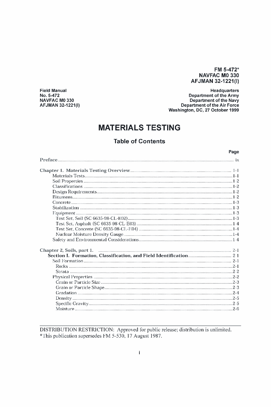
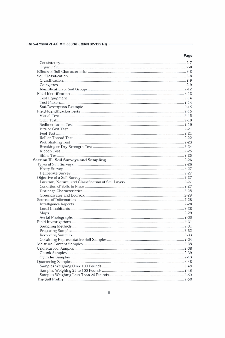
Most Soil Mechanics courses feature a lab course to go with them, either integral or separate. The textbook manufacturers are quick to take advantage of that with expensive books and software. ASTM specs are just about standard in the U.S., but trying to teach out of an ASTM spec is a trying business.
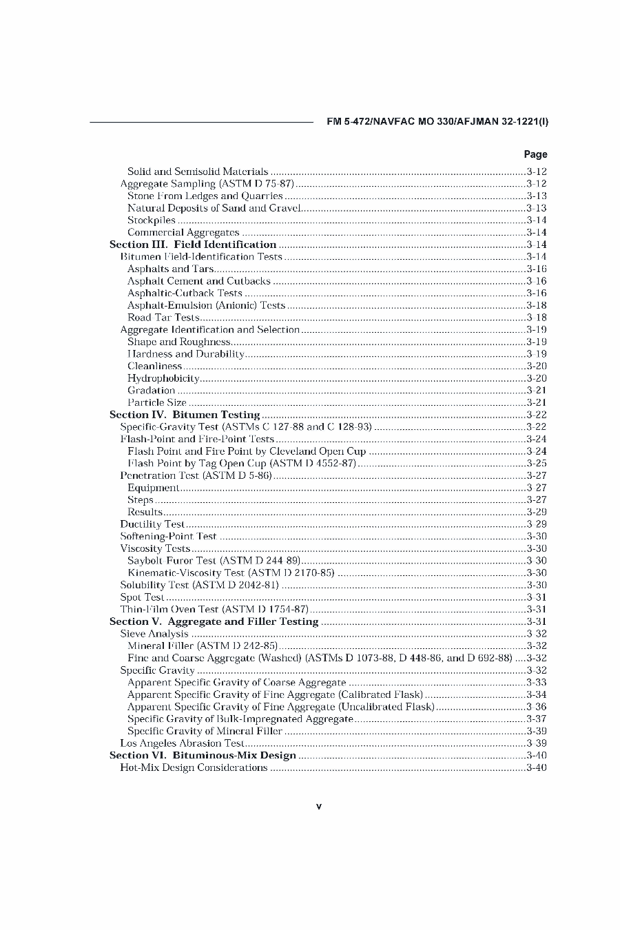
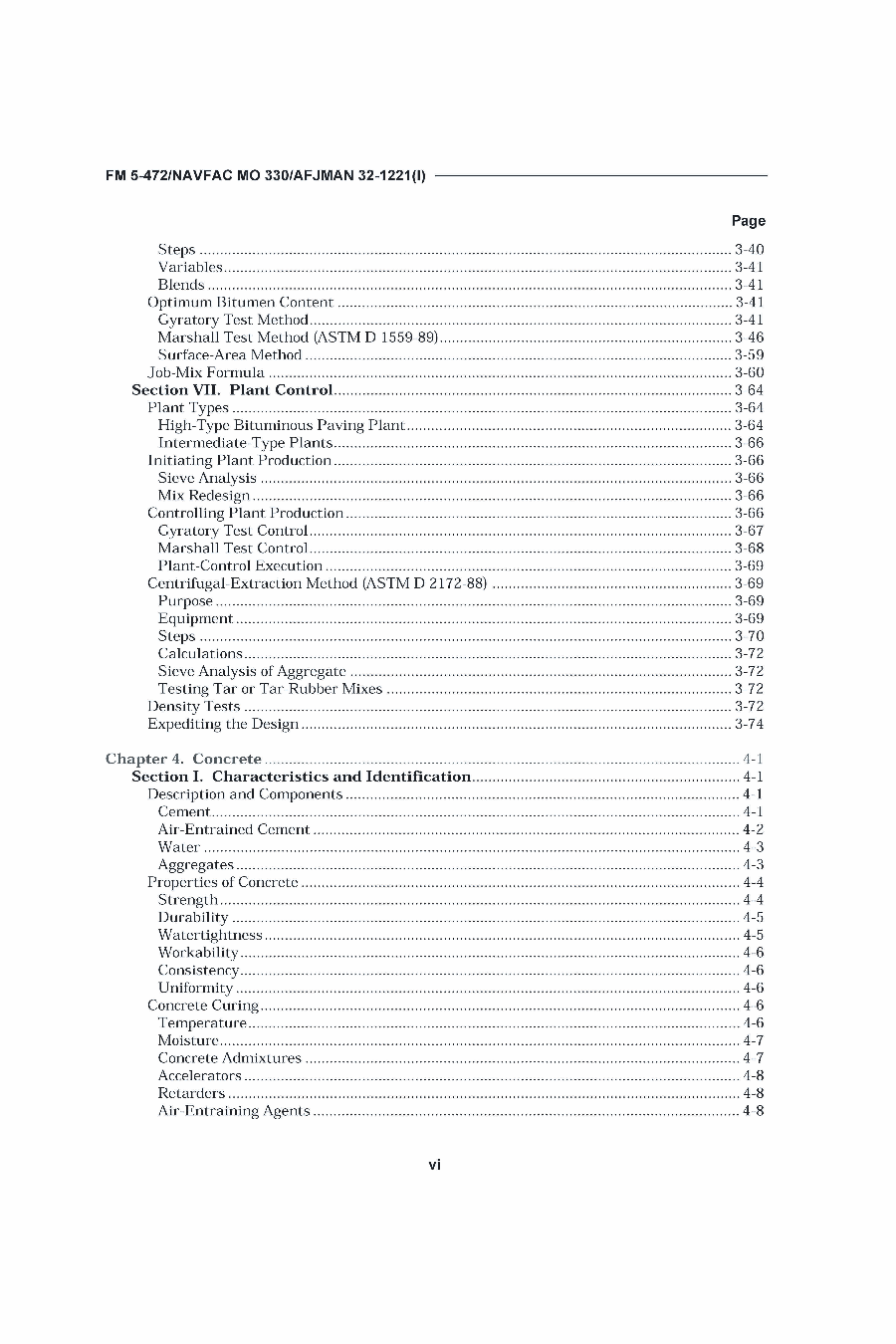
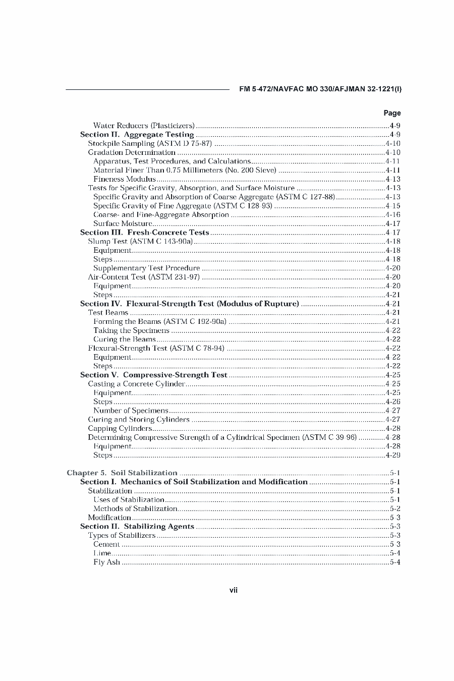
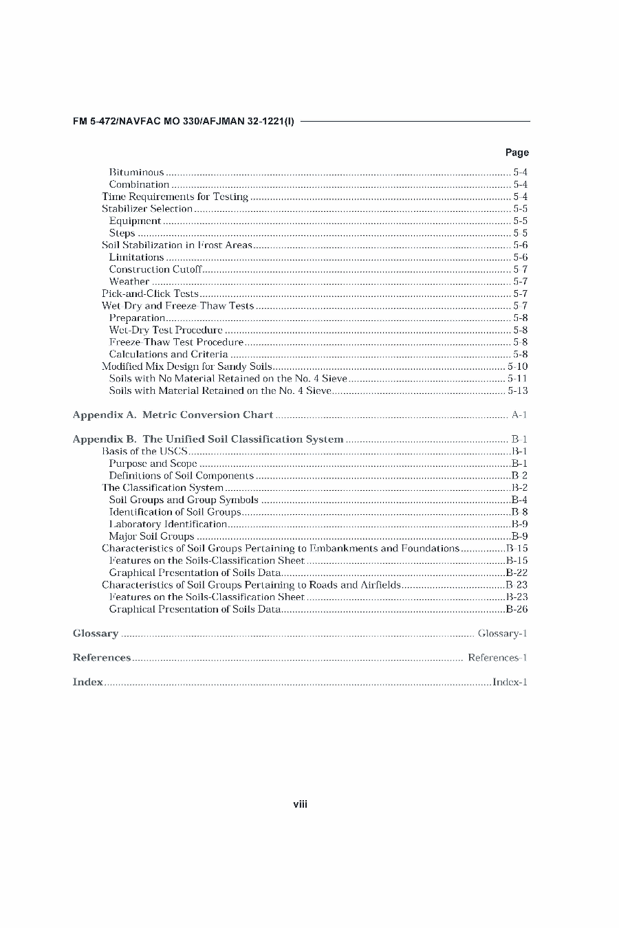
An alternative to this is Materials Testing, the print version of the U.S. Army’s FM 5-472. In addition to the soils tests, it features many other items, some of which are not geotechnical tests at all:
Materials Testing Overview
Soils Testing
Bituminous Mixtures Testing
Concrete Testing
Soil Stabilization
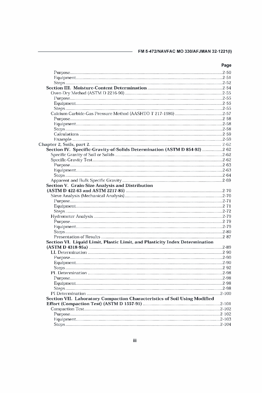
The soils tests in particular are as follows:
Moisture-Content Determination
Specific-Gravity-of-Solids Determination (ASTM D 854-92)
Grain-Size Analysis and Distribution (ASTM D 422-63 and ASTM 2217-85)
Liquid Limit, Plastic Limit, and Plasticity Index Determination (ASTM D 4318-95a)
Laboratory Compaction Characteristics of Soil Using Modified Effort (Compaction Test) (ASTM D 1557-91)
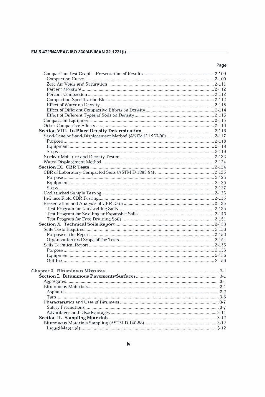
In-Place Density Determination
CBR Tests
You can view the table of contents below.
Materials Testing is an excellent lab manual, supplementary textbook, or handy resource for the testing and improvement of soils, asphalt or concrete.


 can run from 0.9 to 1.15, which would in turn force the load applied by the pile hammer upward more than it would if typical design factors are used. Given the complexity of the loading induced by a hammer during driving, the LRFD equation is generally not employed directly for drivability studies, and the fact that