art – vulcanhammer.net

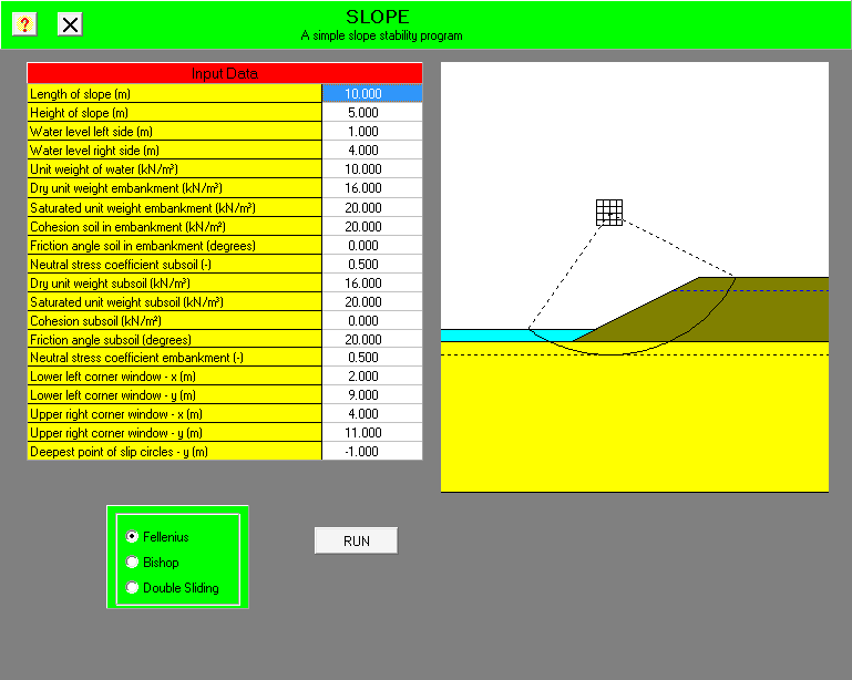
Ever since this site’s predecessor was started in 1997, one of the things it’s “about” is offering useful documents and software at no charge. With software that’s become more difficult as operating systems have changed and some software has become inoperable on newer computer systems. We’ve gotten around that for DOS and Windows 3.1 applications, as shown in Partying Like It’s 1987: Running WEAP87 and SPILE (and other programs) on DOSBox. In this case we’re featuring a Windows-based, 32-bit software program for slope stability called–wait for it–SLOPE. It was developed by the late Arnold Verruijt, whose Soil Mechanics book I used for many years.

Downloading the Software

That’s pretty straightforward: click on the link below and save the file to your computer.

Download SLOPE Stability Software

What you’ll see is slope.zip. Computers and file download sites are getting nervous about raw Windows .exe files, so all you need to do is to extract the one and only slope.exe file from the archive.

Starting SLOPE

Now we come to the first discovery: slope.exe isn’t a program installation file, it is the program! You just double click on it and you will be greeted with the interface shown at the top of the post. The data entry is in the while column under “Input Data.” We will explain the input in an example.

The Example

The example is shown below, it is taken from the Soils and Foundations Reference Manual. The description from there is as follows:

Figure 6-20 shows a 35 ft high slope with a grade of 1.5H:1V. The soil properties within the slope and under it are shown on the figure. Groundwater is immediately under the slope. Calculate the factor of safety for a toe circle by using total stress analysis based on the soil properties shown.

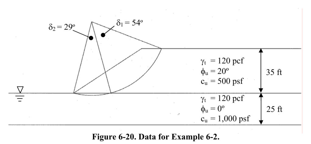
Because slope locates the slip circle of failure, we can ignore the geometry specified in that part of the drawing.

Basic Principle of Operation

SLOPE is based on classical slope stability techniques that goes back to Wolmar Fellenius’ work in the first part of the last century. It assumes that the soil fails along a circular surface, as shown below.

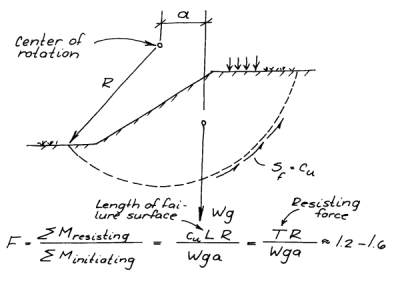
The weight of the soil is driving the soil downward, and this is resisted by the shear resistance along the failure surface (the dashed line.) That resistance is affected by a number of factors, including effective stress along the failure surface, friction of the particles, and cohesion of the soil. The whole mass rotates about the center of rotation, which has to be determined during analysis.

The most common method used–and the one SLOPE uses–is the method of slices. In that method the soil mass is divided into vertical slices, each of which has a mass, some kind of resistance along the failure surface, and (for most of the methods used) how the slices interact with each other.

The theory is described in both Soil Mechanics and the Soils and Foundations Reference Manual. The computations can be laborious, but the really tricky part is determining the location of the center of rotation and the radius R of the failure surface. SLOPE takes care of all of that but it is essential for you to understand how it does that, as its determination of all of these factors is not automatic.

Dealing With Different Expressions of Slope

One common problem with slope stability situations is how the geometry of the slope is defined. There is more than one way of doing it, and the method used in the problem is different than the one used in SLOPE.

The problem states that the slope is 35′ high (the vertical length of the slope) with a grade of 1.5H/1V. This means that, for every foot or meter of height, there are 1.5 feet or meters of horizontal length. In this case the horizontal length is (35)(1.5)/(1) = 52.5′. Alternatively we can compute the angle of slope as arctan(1/1.5) = 33.7 degrees, in which case the length is 35/tan(33.7) = 52.5′

Inputting the Data

SLOPE requires the data to be put in SI units. We will do the conversions as we proceed. The data input is as follows:

Length of slope (m) = 52.5′ = 16 m
Height of slope (m) = 35′ = 10.7 m
Water level left side (m) = 0 (from problem statement, zero is at the toe of the slope)
Water level right side (m) = 0 (again from problem statement)
Unit weight of water (kN/m³) = 10 (reasonable approximation)
Dry unit weight of embankment* (kN/m³) = 120 pcf = 18.9 kN/m³
Saturated unit weight of embankment (kN/m³) = 18.9 (in absence of better data, use the same)
Cohesion soil in embankment (kN/m²) = 500 pcf = 23.9 kN/m²
Friction angle in embankment (degrees) = 20 (from problem statement)
Neutral stress coefficient subsoil** = 1.00
Dry unit weight subsoil* (kN/m³) = 120 pcf = 18.9 kN/m³
Saturated unit weight subsoil (kN/m³) = 18.9 (in absence of better data, use the same)
Cohesion soil subsoil (kN/m²) = 1,000 pcf = 47.9 kN/m²
Friction angle subsoil (degrees) = 0 (from problem statement)
Neutral stress coefficient embankment** = 0.66
Lower left corner window*** – x(m)
Lower left corner window*** – y(m)
Upper right corner window*** – x(m)
Upper right corner window*** – y(m)
Deepest point of slip circles – y(m) = -25′ = -7.6 m (this is negative as it is below the toe of the slope)

Notes:
* The embankment is above the toe. The subsoil is below it.
** The neutral stress coefficient is more commonly referred to in American practice as the at-rest earth pressure coefficients. For normally consolidated soils, it equals to $1 - \sin(\phi)$ , and the results are shown in the input list. The entry points for both are out of order, so be careful.
*** This will be explained below.

Choosing the Window Points and the Method of Analyzing the Slices

If we put all of this data into SLOPE, we get the following result:

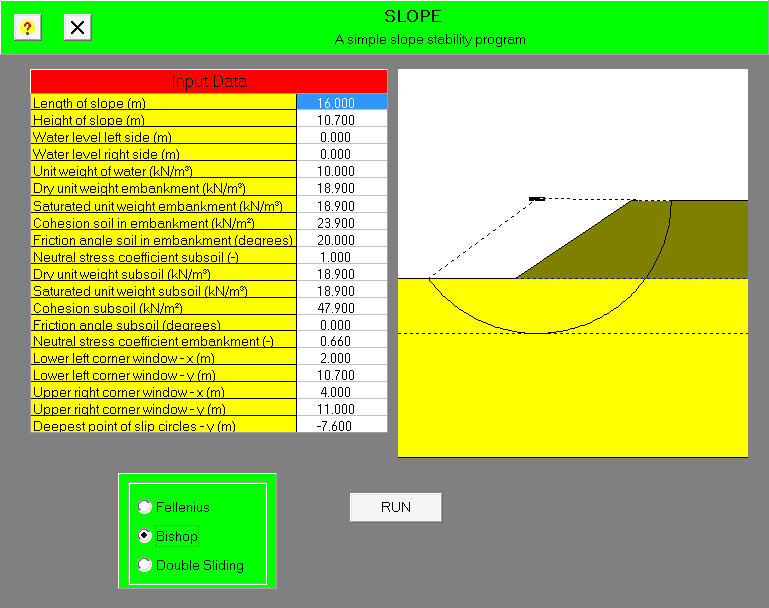
Before we get some results, we have to make two decisions: what slice analysis method to use and the extent of the window.

Soil Mechanics gives an explanation of Fellenius and Bishop’s methods. SLOPE divides the region in the slip circle into the horizontal slices; the difference between these two methods is that Fellenius’ method does not consider friction between the slices while Bishop’s does. Fellenius’ method does not require an iterative solution and is the most conservative; however, given that the computational effort is done by the program, we will use Bishop’s method, which is in common use.

As far as the “window” is concerned, SLOPE, in common with many slope stability programs, uses a grid optimization method to find the location of the rotational centre. This means that a set of points in a regular grid are each analyzed (along with appropriate slip circles) to get the factor of safety (see sketch above) and after analyzing all of these points picks the one with the lowest factor of safety. It’s easy to see that, using the original grid, not much in the way of useful information can be found as the selection of grid points is too small. For a grid point to be valid, it has to be in the interior of the window, not at the edge, because if it’s at the edge it’s possible that the point will be outside of the window.

The window limits are set using a coordinate system with the origin at the toe of the slope. Generally the slip circle centre will be above and to the left of the upper corner of the slope. Values for y should not be less than the slope height and values for x should be greater than zero and less than the length of the slope.

Getting an acceptable result is an iterative process. Let us assume the following for the window boundaries:

Lower left corner window*** – x(m) = 2 m
Lower left corner window*** – y(m) – 10.7 m
Upper right corner window*** – x(m) – 14 m
Upper right corner window*** – y(m) – 15 m

If we apply these and then Bishop’s method for the analysis, we get the following result:

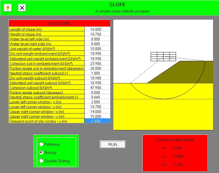
We can see the slip circle centre is in the interior of the grid. If we desire we can shrink the window to get a finer grid and a more precise result.

Sometimes assuming the slip circle going to its lowest point does not result in the lowest factor of safety. To simulate something close to a toe circle, let us set the deepest point at the bottom of the embankment; the result we obtain is as follows:

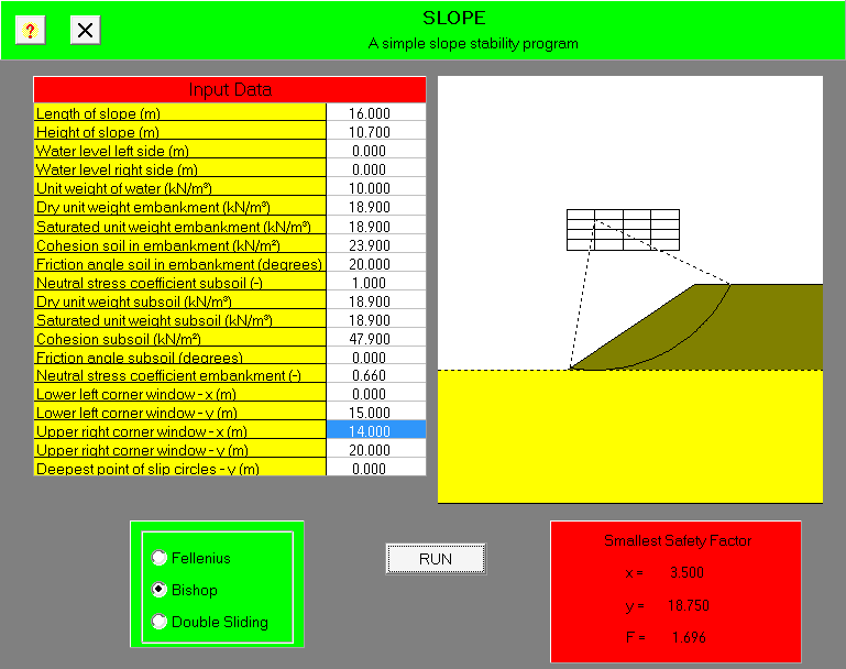
In this case (with some adjustments to the window) the factor of safety is still higher for our original case.

Reporting the Results

SLOPE is not installed, and as a result does not print out its results. The only way to save the results from the program is to get them off of the screen. This is fairly straightforward: use a grab or screenshot program, which was done with the images in this post. Unfortunately many of my students, for whatever reason, insisted on using their phones to take shots of the literal screen, which generally look awful. This was the technology I used forty years ago when presenting this program; we’ve come a long way since.

Conclusion

SLOPE is a fairly simple program to use. It lacks many of the automation and stratigraphy defining features other slope stability software packages have, and is not suited for use in practice. For academic use, however, it is good, and gets students past one of the most tedious features of geotechnical computation.

This is the first of periodic (hopefully not sporadic) articles on the new NAVFAC DM 7.2. In this post I’m going to make some general observations on the book and look at its “Prologue” on shear strength for geotechnical design.

Of the two classic NAVFAC DM 7 volumes, the second–Foundations and Earth Structures–was the “longest in the tooth” largely due to advances in construction technology, and needed upgrading the most. The result of the effort is a long book (721 pages as opposed to 578 in DM 7.1) but one the need for which is greater than 7.1. It also includes some new sections, including one on probabilistic design (LRFD for short) that has been a major change in the way foundations are designed over the last half century.

I’ll get to that later but in the meanwhile here are some general observations:

As was the case with DM 7.1, the graphics are greatly improved, and are up to the standards of their civilian counterparts from the FHWA (which have also been an inspiration to the content of this work.) This is good news, not only for the readers of this book but for those publications which use the graphics in their own books. One of the major upgrades to my and Lee Schroeder’s Soils in Construction was using the FHWA’s better graphics; we had no budget at all for illustrations. It’s always needful to be profitable in business, but textbooks have become cash cows (especially with the major publishers and textbooks) with most of the effort going to places like mastering (which has issues of its own) and not on graphics. For books like Soils in Construction, the graphics will be very helpful. One thing that I held back on was replacing every table and graphic in my Soil Mechanics slides with the new DM 7.1 replacements; I found the older ones, although a lot better looking, to show up better on a screen.
Pursuant to that, any textbook out there needs to be reviewed in reference to both of these volumes, not only for the graphics but to the content. How soon these changes will appear in textbooks depends upon the publisher; I wouldn’t hold my breath, as many textbooks represent “rearranging deck chairs on the Titanic” rather than moving things forward. In the case of this field, we have an advantage, because…
Although DM 7.2 documents many advances in geotechnical engineering, one thing that strikes someone who has followed the history of the profession is struck once again by how conservative this business is. Both volumes get into software solutions but the main audience of both is the geotech who uses formulas (straightforward and otherwise) to achieve their design analysis. This is not to say that this approach is without merit; “black box” technologies are never a good thing from an understanding approach, and can be dangerous when applied indiscriminately. But the nonlinear nature of geotechnical engineering makes some kind of numerical solution (as opposed to a closed form solution) a necessity to deal with the problems geotechnical engineers face. A solution “duo” where closed form solutions (empirical to varying degrees) and numerical ones are used together is the best, and although that’s not the way it’s presented in DM 7.2 it’s a useful guide to put the two together.

Prologue: Shear Strength for Geotechnical Design

The first section of the book isn’t a chapter strictly speaking but is better described as an excursus on the topic of shear strength. My guess (I haven’t as of now discussed the details of this book with its editor) is that it was added due to feedback from DM 7.1; it really belongs in that document.

One of those “conservative” things about both documents is their sticking with Mohr-Coulomb as the “go-to” failure theory in soil mechanics. I discuss this in more depth in My Response to Rodrigo Salgado’s “Forks in the road: decisions that have shaped and will shape the teaching and practice of geotechnical engineering” and an announcement but the bottom line is that, even with all of the alternative failure models that have been developed (such as Cam Clay) none is as widely applicable across the spectrum of soil types as Mohr-Coulomb, and this doesn’t look to change for the foreseeable future.

The prologue chiefly deals with two topics: non-linear failure envelopes and the applicability of different testing methods to different soil conditions. Non-linear failure envelopes have been understood to exist for a long time and get some coverage in the old DM 7 but in this case some additional quantification of these is presented, especially as they relate to “y-intercept” issues of cohesion in various soils when a purely linear failure envelope is used. Application of different testing methods to different soil conditions (including the composition and the drainage state) is helpful; many texts get bogged down on this topic and it’s sometimes hard to figure out how to use the information. In this document the presentation is more concise.

Although it’s probably beyond the authors’ scope on this prologue, there are two topics which could use some further discussion in both of these volumes.

The first is the simple question: what is failure? For most engineered materials the first form of failure considered is yield failure, which is the transition from elastic/path independent behaviour to plastic/path dependent behaviour. With soils how successful this is depends in part upon how elastic the soil is before failure and how sharp the transition is across the failure envelope. There are other ways of dealing with the non-linearity of soils. A hyperbolic model, for example, posits that there really is no failure point; the slope of the line progressively flattens with increasing shear stress. Some soils are amenable to a specific type of modelling and some aren’t. Defining failure also depends upon the application as well.

The second is the issue of dilatancy, which isn’t discussed much in either volume. As detailed in my response to Salgado, this doesn’t get the coverage–or quantification–it deserves in most geotechnical literature, and is one of those things that geotechnical engineers need to be made more aware of. DM 7 was and is a “state of the practice” document, and hopefully by the time our government gets around to revising it again it will take its rightful place in this applied science.