vulcanhammer.net

TAMWAVE 3: Basic Results of Pile Capacity Analysis

Posted on 4 January 201826 May 2025 by Don Warrington

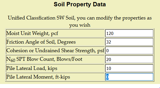
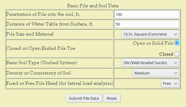
With the soil properties and lateral loads finalised, we can proceed to look at the program’s static results. These are shown below. We will concentrate on cohesionless soils in this post; a sample case with cohesive results will come later.

Pile Data
Pile Designation	12 In. Square
Pile Material	Concrete
Penetration of Pile into the Soil, ft.	100
Basic “diameter” or size of the pile, ft.	1
Cross-sectional Area of the Pile, ft²	1.000
Pile Toe Area, ft²	1.000
Perimeter of the Pile, ft.	4.000
Soil Data
Type of Soil	SW
Specific Gravity of Solids	2.65
Void Ratio	0.51
Dry Unit Weight, pcf	109.5
Saturated Unit Weight, pcf	130.5
Soil Internal Friction Angle phi, degrees	32
Cohesion c, psf	0
SPT N₆₀, blows/foot	20
CPT q_c, psf	211,600
Distance of Water Table from Soil Surface, ft.	50
Penetration of Pile into Water Table, ft.	50
Active Earth Pressure Coefficient (K_min)	0.453
Frictional Angle Between Pile and Soil delta, degrees	27.9
Minimum Value for Beta	0.240
Pile Toe Results
Effective Stress at Pile Toe, ksf	8.880
N_q	22.8
Relative Density at Pile Toe, Percent	40
SPT (N₁)₆₀ at pile toe, blows/foot	10
Unit Toe Resistance q_p, ksf	202.7
Shear Modulus at Pile Toe, ksf	675.7
Toe Spring Constant Depth Factor	1.410
Toe Spring Constant, kips/ft	2,767.9
Pile Toe Quake, in.	0.879
Poisson’s Ratio at Pile Toe	0.310
Toe Damping, kips-sec/ft	13.2
Toe Smith-Type Damping Constant, sec/ft	0.065
Total Static Toe Resistance Q_p, kips	202.67
Pile Toe Plugged?	No
Final Results
Total Shaft Friction Q_s, kips	370.00
Ultimate Axial Capacity of Pile, kips	572.68
Pile Setup Factor	1.0
Total Pile Soil Resistance to Driving (SRD), kips	572.68

Pile Data

The pile data is pretty straightforward. Reproducing it here is an opportunity for you to confirm you’ve selected the correct pile.

Soil Data

Soil data affords the same opportunity for verification; however, it also shows the way the soil data is interpreted to generate the necessary parameters for shaft and toe resistance to load, both static and dynamic.

The first thing that is shown is assumed specific gravity and void ratio. TAMWAVE assumes cohesionless soils have a particle specific gravity of 2.65 and for cohesive soils 2.7. The void ratio is then computed using basic soil mechanics formulae. To do this it is necessary to know the unit weight. The typical properties tables show this in two ways. For cohesionless soils, the “moist” unit weight is shown, and for cohesive soils the saturated unit weight is shown. In both cases this is reduced to dry and saturated unit weights by assuming that S=50% for the cohesionless soils and S=100% for the cohesive ones. Thus, for cohesionless soils neither value will be the same as given in the typical properties.

The internal friction angle, cohesion and $N_{60}$ values are taken from the typical properties as modified (or not) by the user. The equivalent $q_c$ is also reported here, based on the Robertson and Campanella research as reported by Fellenius. As noted earlier, neither the $N_{60}$ values nor the $q_c$ values are actually used in the analysis.

Finally we get to the data necessary to compute the shaft friction. The methods used in TAMWAVE for ultimate shaft resistance are as follows:

Cohesionless soils: Randolph, Dolwin and Beck (1994), which are described here
Cohesive soils: Kolk and van der Velde (1996), which are described here

For cohesionless soils, it is necessary to compute the minimum/active earth pressure coefficient, which of course is strictly a function of $\phi$ . Discussion of $K_{act}$ brings us to the issue of computing $\beta$ . In this post $\beta$ was initially computed using the following formula

$\beta = K tan \phi$

However, as pointed out in the same place, both retaining wall practice and empirical pile capacity formulae show that the friction angle between the wall/pile shaft and the soil is not equal to the internal friction angle of the soil, and so this formula should really be written as

$\beta = K tan \delta$

This actually has a theoretical basis, and in fact is one of the knottiest problems in theoretical soil mechanics. We can consider this by considering the failure along the pile surface as a “direct shear” type of failure, where failure is induced along a predetermined surface. For the case where the principal stresses are normal and tangential to the surface (which is generally the case with driven piles) the failure surface predicted by Mohr’s circle and Mohr-Coulomb theory is not the same as the “predetermined” surface. The most acrimonious manifestation of this problem was with the shear failure of cellular cofferdams, which led to the dispute between Karl Terzaghi and Dmitri Krynine.

Although various studies have been made to determine friction on an empirical basis, probably the simplest solution, suggested by Šuklje (1969), is to compute the apparent friction angle by the formula

$\delta = tan^{-1} (sin \phi)$

Using this result and the active earth pressure coefficient, the minimum value for $\beta$ is readily computed.

Pile Toe Results

Now we get to the application of these parameters. The decision to not use equivalent CPT values has two immediate results. The first is that the unit toe resistance is most easily computed (for cohesionless soils) by the equation

$q_t = N_q \sigma'_{vo}$

Use of bearing capacity factors for toe resistance is both well embedded in literature and practice and well criticised in the same place. Additionally it is necessitated by the fact that the shaft friction is dependent upon $N_q$ , as discussed here.

So what value of $N_q$ should we adopt? As is all too common in geotechnical engineering, there has been a proliferation of values for this parameter. We experimented with several, including that of Vesic (1977). In addition to the usual theortical vs. empirical (and all the variations in between) divide, another factor is whether provision for soil elasticity is taken into consideration. Although methods such as Vesic (1977) do this, their main weakness is their tendency to be stiff, thus returning unrealistically high values of $N_q$ . Taking into account both theoretical methods and empirical ones such as Dennis and Olson, the first method tried for TAMWAVE was from Verruijt), namely:

$N_{\sigma} = K_p e^{\pi tan \phi}$

Note that we’re not at $N_q$ quite yet. For reasons explained by Vesic (1977), the pile toe unit resistance should be a function of $\frac {I_1}{3}$ . (An explanation of this quantity can be found here.) Thus,

$N_q = K_p e^{\pi tan \phi} \frac {I_1}{3 \sigma'_{vo}}$

If we use Jaky’s Equation for normally consolidated soils for the pile toe condition (we will definitely change this for the shaft,)

$\frac {I_1}{3 \sigma'_{vo}} = 1 - \frac {2}{3} sin \phi$

and so

$q_t = K_p e^{\pi tan \phi} \left( 1 - \frac {2}{3} sin \phi \right) \sigma'_{vo}$

This method yields conservative values of $N_q$ . It only takes into consideration the plasticity of the soil, and is additionally subject to the criticism of the entire concept of “bearing capacity” at the pile toe. Given this, a different (and more empirical) approach based on Randolph, Dolwin and Beck (1994) was chosen, which estimates the bearing capacity coefficient as follows:

$N_q=\frac{0.065S+25}{\left( \frac{\sigma'_{vo}}{p_{atm}} \right)^{0.25}}$

$S$ is the coefficient from the Hardin and Black (1968) method of estimating the shear modulus of the soil (see below.) Although this coefficient varies with silt content, for TAMWAVE we will assume $S = 315$ , thus this reduces to

$N_q=\frac{45.475}{\left( \frac{\sigma'_{vo}}{p_{atm}} \right)^{0.25}}$

If static capacity were our sole interest, we would be done with toe. But what about its response to movement? For both toe and shaft resistance, in both static and dynamic cases, we intend to use an elastic-purely plastic model. Assuming no preloading of the system, there are only two parameters we need to know: the ultimate/purely plastic resistance of the soil, and the deflection at which we reach that resistance. The spring constant can be computed by dividing the ultimate resistance by that deflection, or conversely we can determine that deflection by dividing the resistance by a known spring constant. It is the latter operation we will use in TAMWAVE, which leaves us to determine the spring constant of the toe and eventually along the shaft.

We will have occasion to return to this topic, but to determine spring constants we will use the model of Randolph and Simons (1985). For the toe this in turn is dependent upon Lysmer’s Analogue; both of these are discussed in detail in Warrington (1997). They are dependent upon determining values for the soil shear modulus $G$ . (They are also dependent upon the dry unit weight $\gamma$ and Poisson’s Ratio $\nu$ , but both of these parameters are known from basic soil properties and, indirectly, through Jaky’s Equation.) That in turn brings us to another “sticky wicket,” namely determining the shear (or for that matter the elastic) modulus of the soil. An interesting discussion of this topic can be found in Salgado, Loukidis, Abou-Jaoude and Zhang (2015). Assuming a hyperbolic type of soil deformation, there are two basic extremes to this parameter:

The small-strain (or tangent) value, the highest possible value.
The large-strain (or secant) value, the lowest possible value.

Based on their review of the literature, they conclude that the value for (2) can be 10-50% of (1). Although this problem is frought with uncertainties, it is hard to avoid the conclusion that this is a substantial spread and, for our purposes, raises as many questions as it answers. The “solution” to this problem is found in this post, where one attempts to define a ratio between (1) and (2) based on some consideration of anticipated deflections under load for a given application.

Based on some experimentation with the code and earlier considerations, we decided to use a ratio between the two of 0.15, i.e., the secant modulus used in elastic-purely plastic models is 15% of the tangent modulus from the hyperbolic model. We should emphasise that this is not “set in stone” but subject to variation. One of the advantages of a project such as TAMWAVE is the ability to alter parameters and see the results without affecting results on actual projects.

“Fixing” this ratio allows us to determine the shear modulus based on the tangent or small-strain value, and this can be computed by the method proposed in Hardin and Black (1968). There is little difference between the correlation for cohesionless and cohesive soils. There are many ways of expressing this; the one we used (for values of $G$ in psf) is as follows:

$G=S p_{atm}\frac{\left(3-e\right)^{2}}{1+e}\sqrt{\frac{\sigma'_{vo}}{p_{atm}}\frac{1+2K}{3}}$

As before, for TAMWAVE (and many applications) $S = 315$ . The same formula is used for the shaft friction, the main difference is that the lateral earth pressure coefficient is different thus the lateral/confining stresses are different. At the toe we use the result from Jaky’s Equation, which was explained in Verruijt’s method above.

Once this is computed, the pile toe stiffness is computed. The stiffness is increased by multiplying it by a depth factor (Salgado, Loukidis, Abou-Jaoude and Zhang (2015)

$D_f = 1+\left( 0.27- 0.12 ln \nu \right)\left\{ 1-e^{\left[ -0.83\left( \frac{D}{B} \right)^{0.83} \right]} \right\}$

Even at this, when compared to “conventional” toe quakes in dynamic analysis, the toe quake shown above seems rather large. We will leave this as it is for the static analysis and will return to this topic with the dynamic analysis.

Since we are computing stiffnesses for shaft and toe here, we will also do the same for damping. Traditionally wave equation programs have used “Smith damping,” but as we will see this will be modified for the wave equation analysis. To start let us redefine the “Smith type damping constant” as

$j = \frac {\mu}{R_u}$

In this case $\mu$ is the damping constant for the toe or shaft element in question, computed using the formulae given in Warrington (1997). $R_u$ is the ultimate resistance of the toe or shaft element in question. The toe damping constant that results in this case is somewhat lower than “standard” values; this will be discussed later.

Final Results

The final results are at the end of the table. The shaft friction computation will be discussed in the next post. The cohesive calculations have a provision for pile set-up using cavity expansion theory and this will be discussed later.

References

In addition to works already cited in this and the STADYN study, the following should be noted:

Hardin, B.O., and Black, W.L. (1968). “Vibration modulus of normally consolidated clay.” J. Soil Mech. Found. Div. 94, No. 2, 353-370.
Salgado, R., Loukidis, D., Abou-Jaoude, G., and Zhang, Y. (2015) “The role of soil stiffness non-linearity in 1D pile driving simulations.” Geotechnique 65, No. 3, 169-187. http://dx.doi.org/10.1680/geot.13.P.124
Vesic, A.S. (1977) Design of Pile Foundations. NCHRP Synthesis 42. Washington, DC: Transportation Research Board.

TAMWAVE

TAMWAVE 2: Modifying the Soil Properties

Posted on 3 January 201826 May 2025 by Don Warrington

With the first step out of the way, we can proceed to the second: allowing the user to modify the properties of the soil. This option must be used with care since it is easily possible to put together a set of soil properties that is physically unrealistic if not impossible.

Also, if you have chosen a sand or clay, you have chosen the methodology you will use. Adding cohesion to a sand or gravel, for example, will have no effect on the subsequent performance of the model.

Finally, depending upon the choice of a free or fixed head, you are given the option of entering lateral loads and/or moments for the pile head. In this case we have opted to add a lateral load of 10 kips to the pile and no moment. The default is zero for both load and moment; this will produce some coefficients but no result for lateral loading.

Once the properties are as required, you can accept the form and proceed to the next step.

TAMWAVE

TAMWAVE 1: Entering Basic Soil and Pile Properties

Posted on 3 January 201826 May 2025 by Don Warrington

With a few preliminaries out of the way, we can proceed to discuss the new TAMWAVE routine, which can be found here.

What is TAMWAVE?

TAMWAVE stands for Texas A&M Wave Equation. The TTI wave equation was developed at Texas A&M in the late 1960’s and early 1970’s, and was a successor to Smith’s original wave equation program. In reality this is more than a wave equation program; it is a driven pile analyser which, in addition to the wave equation program, analyses the static performance of a driven pile for both axial and lateral loads. It is not intended to be used on actual projects, but as an educational tool for students. Most of the software in current use is expensive, and predecessors such as SPILE, WEAP87 or COM624 are hard to use (they’re DOS programs) or methodological obsolescence issues. (With WEAP87, there are not as many of those as you might think, but that’s another post…)

Limitations of TAMWAVE

Given that this is an educational tool, there are some significant limitations to TAMWAVE’s capabilities. Some of these are as follows:

Only one type and consistency/density of soil is permitted. However, the phreatic surface can be anywhere between the head and toe of the pile. (If at the toe, the soil is assumed to be dry for the entire length of the pile, an unlikely scenario.)
Piles have uniform cross-section and material for the entire length. Starting in 2010, piles must be picked from a database presented at the start of the routine. This limits the types of piles available, but makes input a lot simpler.
Hammers are likewise limited to air/steam hammers, currently Vulcan and Raymond models. (We may add Conmaco ones, later.) This excludes diesel and hydraulic impact hammers, which simplifies the code considerably.
Both axial and lateral loads are analysed by assuming the soil is either completely cohesionless or cohesive. Unfortunately this is also a limitation of most current driven pile analysis methods as well. Generally speaking, soils are entirely neither, but they’re close enough for current methods. We’ll explore how to deal with this in the STADYN project; for now, we’ll stick with the binary methodology.

Test Case, and Entering the Data

For this series of explanations we’ll use a test case as follows:

12″ concrete pile
100′ long (all piles are groundline in TAMWAVE, so there is no “stick-up” permitted
Water table 50′ below surface
Soil cohesionless or cohesive; in both cases a “medium” soil

Starting with the initial page, the data form looks like this:

The pile data input is pretty straightforward; the option for closed or open-ended pile toe is only relevant for hollow piles (pipe or concrete cylinder piles.) The soil type is entered using the two-letter Unified system code. This is to accomplish two things:

To make it simple to match the soil description from boring logs, if the problem is stated using one; and
In the case of cohesionless soils, to vary the internal friction angle with the soil type.

Density or consistency choice depends upon whether the soil is cohesionless or cohesive; the following charts (from here) were used for the data:

This slideshow requires JavaScript.

At this point we need to pause and consider something we discussed in our last post: the use of CPT data.

When we attempt to establish soil response to load our ultimate goal is to determine the engineering properties of the soil. Assuming we’re still in a Mohr-Coulomb universe, and setting aside the issue of consolidation settlement, that means three properties: the internal friction angle $\phi$ , the cohesion $c$ , and the unit weight (dry, moist or saturated) $\gamma$ . Ideally we can establish these properties using undisturbed samples in the laboratory. The tricky part comes in obtaining these samples: not only is it expensive, but getting a truly “undisturbed” sample out of the soil is next to impossible, although we can come close. This is why, from the earliest years of geotechnical engineering as a science, we’ve resorted to either tests of disturbed samples (the Atterberg limits are the most prominent of these) or in situ tests such as SPT, CPT or vane shear. In the United States the SPT test has pretty much reigned supreme and is still the most commonly used test, in spite of its manifest limitations and inconsistencies, and appears on many soil boring logs.

Unfortunately most of the “academic” work in pile capacity has centred on the use of CPT results. It was the original idea to essentially convert the SPT results from the charts above to “typical” CPT results and then use these with more contemporary techniques. Unfortunately, in the development of TAMWAVE, it became clear that the results from doing this–especially with the toe response–had problems. Based on this, we decided to drop the use of the artificially generated CPT data and use methods which could be derived from other properties. The reason for this is twofold: the buildup of pore water pressures around the cone tip during insertion made the relationship between $q_c$ and $q_t$ problematic, and this, combined with basic differences in the SPT and CPT methodologies, makes correlating the two not a straightforward proposition. These are discussed in and the geotechnical practitioner would do well to keep this in mind when dealing with the results of either test.

One good thing that resulted from this decision is that we did not have much recourse to the SPT “data” either. We were able to use the “Mohr-Coulomb” triple directly for most of our calculations.

The last piece of data is for lateral piles only: it is whether the head of the pile is “fixed” or “free” for lateral load analysis. The loads themselves will be entered in the next step, which is accomplished by completing the for and pressing the “Submit Pile Data” button.

Uncategorized

Argument from authority

Posted on 29 December 2017 by Don Warrington

The Logical Place

by Tim Harding

The Argument from Authority is often misunderstood to be a fallacy in all cases, when this is not necessarily so. The argument becomes a fallacy only when used deductively, or where there is insufficient inductive strength to support the conclusion of the argument.

The most general form of the deductive fallacy is:

Premise 1: Source A says that statement p is true.
Premise 2: Source A is authoritative.
Conclusion: Therefore, statement p is true.

Even when the source is authoritative, this argument is still deductively invalid because the premises can be true, and the conclusion false (i.e. an authoritative claim can turn out to be false).[1] This fallacy is known as ‘Appeal to Authority’.

The fallacy is compounded when the source is not an authority on the relevant subject matter. This is known as Argument from false or misleading authority.

Although reliable…

View original post 475 more words

Geotechnical Engineering, Soil Mechanics, STADYN, TAMWAVE

Relating Hyperbolic and Elasto-Plastic Soil Stress-Strain Models

Posted on 2 December 201726 May 2025 by Don Warrington

Note: this post has an update to it with a more rigourous and complete treatment here.

It is routine in soil mechanics to attempt to use continuum mechanics/theory of elasticity methods to analyse the stresses and strains/deflections in soil. We always do this with the caveat that soils are really not linear in their response to stress, be that stress axial, shear or a combination of the two. In the course of the STADYN project, that fact became apparent when attempting to establish the soil modulus of elasticity. It is easy to find “typical” values of the modulus of elasticity; applying them to a given situation is another matter altogether. In this post we will examine this problem from a more theoretical/mathematical side, but one that should vividly illustrate the pitfalls of establishing values of the modulus of elasticity for soils.

Although the non-linear response of soils can be modelled in a number of ways, probably the most accepted method of doing so is to use a hyperbolic model of soil response. This is illustrated (with an elasto-plastic response superimposed in red) below.

The difficulties of relating the two curves is apparent. The value E1 is referred to as the “tangent” or “small-strain” modulus of elasticity. (In this diagram axial modulus is shown; similar curves can be constructed for shear modulus G as well.) This is commonly used for geophysical methods and in seismic analyses.

As strain/deflection increases, the slope of the curve decreases continuously, and the tangent modulus of elasticity thus varies continuously with deflection. For larger deflections we frequently resort to a “secant” modulus of elasticity, where we basically draw a line between the origin (usually) and whatever point of strain/deflection we are interested in.

Unfortunately, like its tangent counterpart, the secant modulus varies too. The question now arises: what stress/strain point do we stop at to determine a secant modulus? Probably a better question to ask is this: how do we construct an elasto-plastic curve that best fits the hyperbolic one?

One solution mentioned in the original study is that of Nath (1990), who used a hardening model instead of an elastic-purely plastic model. The difference between the two is illustrated below.

Although this has some merit, the elastic-purely plastic model is well entrenched in the literature. Moreover the asymptotic nature of the hyperbolic model makes such a correspondence “natural.”

Let us begin by making some changes in variables. Referring to the first figure,

$y=\frac{\sigma}{\sigma_1-\sigma_3}=\frac{\sigma}{\sigma_0}$

and

$x = \epsilon$

Let us also define a few ratios, thus:

$A_1 = \frac {E_1}{\sigma_0}$

$A_2 = \frac {E_2}{\sigma_0}$

$A = \frac {E_2}{E_1}$

Substituting these into the hyperbolic equation shown above, and doing some algebra, yields

$y=\frac{x A_1}{1+x A_1}$

One way of making the two models “close” to each other is to use a least-squares (2-norm) difference, or at least minimising the 1-norm difference. To do the latter with equally spaced data points is essentially to minimise the difference (or equate if possible) the integrals of the two, which also equates the strain energy. This is the approach we will take here.

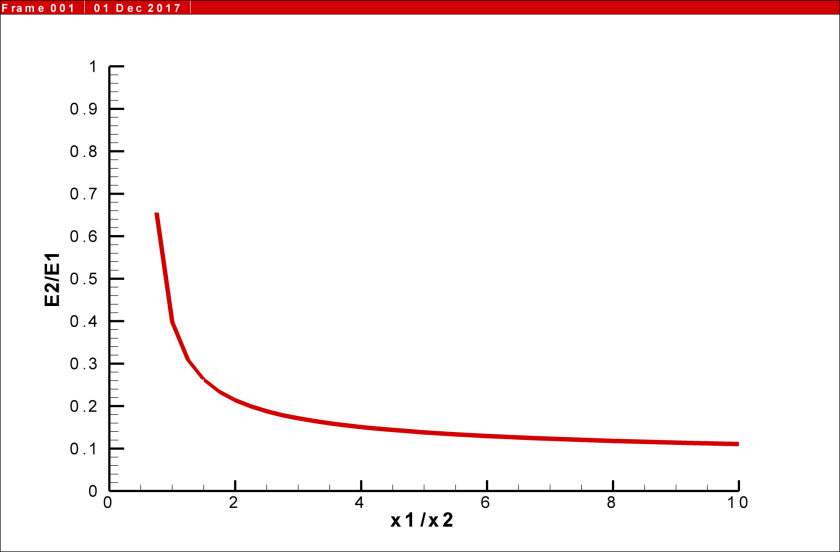
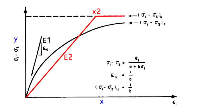
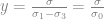
It is easier to equate the areas between the two curves and the $\sigma_0$ line than to the x-axis. To do this we need first to rewrite the previous equation as

$y'=1-\frac{x A_1}{1+x A_1}$

Integrating this with respect to $x$ from 0 to some value $x_1$ yields

$A_{hyp} = \frac{ln\left( 1+x_1 A_1 \right)}{A_1}$

Turning to the elastic-plastic model, the area between this “curve” and the maximum stress is simply the triangle area above the elastic region. Noting that

$E_2 = \frac {\sigma_0} {x_2}$ ,

employing the dimensionless variables defined above and doing some additional algebra yields the area between the elastic line and the maximum stress, which is

$A_{ep} = \frac {1}{2 A A_1}$

Equation the two areas, we have

$ln\left( 1+x_1 A_1 \right) - \frac {1}{2 A} = 0$

With this equation, we have good news and bad news.

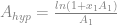
The good news is that we can (or at least think we can) solve explicitly for $A$ , the ratio between the elastic modulus needed by elasto-plastic theory and the small-deflections modulus from the hyperbolic model. The bad news is that we need to know $A_1$ , which is the ratio of the small deflections modulus to the limiting stress. This implies that the limiting stress will be a factor in our ultimate result. Even worse is that $x_1$ is an input variable, which means that the result will depend upon how far we go with the deflection.

This last point makes sense if we consider the two integrals. The integral for the elasto-plastic model is bounded; that for the hyperbolic model is not because the stress predicted by the hyperbolic model is asymptotic to the limiting stress, i.e., it never reaches it. This is a key difference between the two models and illustrates the limitations of both.

Some additional simplification of the equation is possible, however, if we make the substitution

$x_1 = n x_2$

In this case we make the maximum strain/deflection a multiple of the elastic limit strain/deformation of the elasto-plastic model. Since

$x_2 = \frac {sigma_0}{E_2} = \frac {1}{A_2} = \frac {1}{A A_1}$

we can substitute to yield

$ln\left( 1+\frac{n}{A} \right) - \frac{1}{2A} = 0$

At this point we have a useful expression which is only a function of $n$ and $A$ . The explicit solution to this is difficult; the easier way to do this is numerically. In this case we skipped making an explicit derivative and use regula falsi to solve for the roots for various cases of $n$ . Although this method is slow, the computational time is really trivial, even for many different values of $n$ . The larger value of $n$ , the more deflection we are expecting in the system.

The results of this survey are shown in the graph below.

The lowest values we obtained results for were about $n = \frac{x_1}{x_2} = 0.75$ . When $n = \frac{x_1}{x_2} = 1$ , it is the case when the anticipated deflection is approximately equal to the “yield point.” For this case the ratio between the elasto-plastic modulus and the small-strain hyperbolic modulus is approximately 0.4. As one would expect, as $n$ increases the elasto-plastic system becomes “softer” and the ratio $A = \frac {E_2}{E_1}$ likewise decreases. However, as the deflection increases this ratio’s increase is not as great.

To use an illustration, consider pile toe resistance in a typical wave equation analysis. Consider a pile where the quake ( $x_2$ ) is 0.1″. Most “traditional” wave equation programs estimate the permanent set per blow to be the maximum movement of the pile toe less the quake. In the case of 120 BPF–a typical refusal–the set is 0.1″, which when added to the quake yields a total deflection of 0.2″ of a value of $n = 2$ . This implies a value of $A = 0.2139950$ . On the other hand, for 60 BPF, the permanent set is 0.2″, the total movement is 0.3″, and $n = 3$ , which implies a value of $A = 0.1713409$ . Cutting the blow count in half again to 30 BPF yields $n = 5$ or $A = 0.1383195$ . Thus, during driving, not only does the plastic deformation increase, the effective stiffness of the toe likewise decreases as well.

Based on all this, we can draw the following conclusions:

The ratio between the equivalent elasto-plastic modulus and the small-strain modulus decreases with increasing deflection, as we would expect.
As deflections increase, the effect on the the equivalent modulus decreases.
Any attempt to estimate the shear or elastic modulus of soils must take into consideration the amount of plastic deformation anticipated during loading. Use of “typical” values must be tempered by the actual application in question; such values cannot be accepted blindly.
The equivalence here is with hyperbolic soil models. Although the hyperbolic soil model is probably the most accurate model currently in use, it is not universal with all soils. Some soils exhibit a more definite “yield” point than others; this should be taken into consideration.