Relating Hyperbolic and Elasto-Plastic Soil Stress-Strain Models

Note: this post has an update to it with a more rigourous and complete treatment here.

It is routine in soil mechanics to attempt to use continuum mechanics/theory of elasticity methods to analyse the stresses and strains/deflections in soil. We always do this with the caveat that soils are really not linear in their response to stress, be that stress axial, shear or a combination of the two. In the course of the STADYN project, that fact became apparent when attempting to establish the soil modulus of elasticity. It is easy to find “typical” values of the modulus of elasticity; applying them to a given situation is another matter altogether. In this post we will examine this problem from a more theoretical/mathematical side, but one that should vividly illustrate the pitfalls of establishing values of the modulus of elasticity for soils.

Although the non-linear response of soils can be modelled in a number of ways, probably the most accepted method of doing so is to use a hyperbolic model of soil response. This is illustrated (with an elasto-plastic response superimposed in red) below.

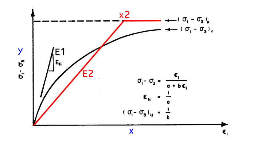
The difficulties of relating the two curves is apparent. The value E1 is referred to as the “tangent” or “small-strain” modulus of elasticity. (In this diagram axial modulus is shown; similar curves can be constructed for shear modulus G as well.) This is commonly used for geophysical methods and in seismic analyses.

As strain/deflection increases, the slope of the curve decreases continuously, and the tangent modulus of elasticity thus varies continuously with deflection. For larger deflections we frequently resort to a “secant” modulus of elasticity, where we basically draw a line between the origin (usually) and whatever point of strain/deflection we are interested in.

Unfortunately, like its tangent counterpart, the secant modulus varies too. The question now arises: what stress/strain point do we stop at to determine a secant modulus? Probably a better question to ask is this: how do we construct an elasto-plastic curve that best fits the hyperbolic one?

One solution mentioned in the original study is that of Nath (1990), who used a hardening model instead of an elastic-purely plastic model. The difference between the two is illustrated below.

Although this has some merit, the elastic-purely plastic model is well entrenched in the literature. Moreover the asymptotic nature of the hyperbolic model makes such a correspondence “natural.”

Let us begin by making some changes in variables. Referring to the first figure,

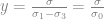
$y=\frac{\sigma}{\sigma_1-\sigma_3}=\frac{\sigma}{\sigma_0}$

and

$x = \epsilon$

Let us also define a few ratios, thus:

$A_1 = \frac {E_1}{\sigma_0}$

$A_2 = \frac {E_2}{\sigma_0}$

$A = \frac {E_2}{E_1}$

Substituting these into the hyperbolic equation shown above, and doing some algebra, yields

$y=\frac{x A_1}{1+x A_1}$

One way of making the two models “close” to each other is to use a least-squares (2-norm) difference, or at least minimising the 1-norm difference. To do the latter with equally spaced data points is essentially to minimise the difference (or equate if possible) the integrals of the two, which also equates the strain energy. This is the approach we will take here.

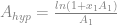
It is easier to equate the areas between the two curves and the $\sigma_0$ line than to the x-axis. To do this we need first to rewrite the previous equation as

$y'=1-\frac{x A_1}{1+x A_1}$

Integrating this with respect to $x$ from 0 to some value $x_1$ yields

$A_{hyp} = \frac{ln\left( 1+x_1 A_1 \right)}{A_1}$

Turning to the elastic-plastic model, the area between this “curve” and the maximum stress is simply the triangle area above the elastic region. Noting that

$E_2 = \frac {\sigma_0} {x_2}$ ,

employing the dimensionless variables defined above and doing some additional algebra yields the area between the elastic line and the maximum stress, which is

$A_{ep} = \frac {1}{2 A A_1}$

Equation the two areas, we have

$ln\left( 1+x_1 A_1 \right) - \frac {1}{2 A} = 0$

With this equation, we have good news and bad news.

The good news is that we can (or at least think we can) solve explicitly for $A$ , the ratio between the elastic modulus needed by elasto-plastic theory and the small-deflections modulus from the hyperbolic model. The bad news is that we need to know $A_1$ , which is the ratio of the small deflections modulus to the limiting stress. This implies that the limiting stress will be a factor in our ultimate result. Even worse is that $x_1$ is an input variable, which means that the result will depend upon how far we go with the deflection.

This last point makes sense if we consider the two integrals. The integral for the elasto-plastic model is bounded; that for the hyperbolic model is not because the stress predicted by the hyperbolic model is asymptotic to the limiting stress, i.e., it never reaches it. This is a key difference between the two models and illustrates the limitations of both.

Some additional simplification of the equation is possible, however, if we make the substitution

$x_1 = n x_2$

In this case we make the maximum strain/deflection a multiple of the elastic limit strain/deformation of the elasto-plastic model. Since

$x_2 = \frac {sigma_0}{E_2} = \frac {1}{A_2} = \frac {1}{A A_1}$

we can substitute to yield

$ln\left( 1+\frac{n}{A} \right) - \frac{1}{2A} = 0$

At this point we have a useful expression which is only a function of $n$ and $A$ . The explicit solution to this is difficult; the easier way to do this is numerically. In this case we skipped making an explicit derivative and use regula falsi to solve for the roots for various cases of $n$ . Although this method is slow, the computational time is really trivial, even for many different values of $n$ . The larger value of $n$ , the more deflection we are expecting in the system.

The results of this survey are shown in the graph below.

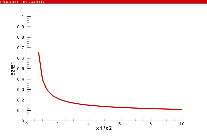
The lowest values we obtained results for were about $n = \frac{x_1}{x_2} = 0.75$ . When $n = \frac{x_1}{x_2} = 1$ , it is the case when the anticipated deflection is approximately equal to the “yield point.” For this case the ratio between the elasto-plastic modulus and the small-strain hyperbolic modulus is approximately 0.4. As one would expect, as $n$ increases the elasto-plastic system becomes “softer” and the ratio $A = \frac {E_2}{E_1}$ likewise decreases. However, as the deflection increases this ratio’s increase is not as great.

To use an illustration, consider pile toe resistance in a typical wave equation analysis. Consider a pile where the quake ( $x_2$ ) is 0.1″. Most “traditional” wave equation programs estimate the permanent set per blow to be the maximum movement of the pile toe less the quake. In the case of 120 BPF–a typical refusal–the set is 0.1″, which when added to the quake yields a total deflection of 0.2″ of a value of $n = 2$ . This implies a value of $A = 0.2139950$ . On the other hand, for 60 BPF, the permanent set is 0.2″, the total movement is 0.3″, and $n = 3$ , which implies a value of $A = 0.1713409$ . Cutting the blow count in half again to 30 BPF yields $n = 5$ or $A = 0.1383195$ . Thus, during driving, not only does the plastic deformation increase, the effective stiffness of the toe likewise decreases as well.

Based on all this, we can draw the following conclusions:

The ratio between the equivalent elasto-plastic modulus and the small-strain modulus decreases with increasing deflection, as we would expect.
As deflections increase, the effect on the the equivalent modulus decreases.
Any attempt to estimate the shear or elastic modulus of soils must take into consideration the amount of plastic deformation anticipated during loading. Use of “typical” values must be tempered by the actual application in question; such values cannot be accepted blindly.
The equivalence here is with hyperbolic soil models. Although the hyperbolic soil model is probably the most accurate model currently in use, it is not universal with all soils. Some soils exhibit a more definite “yield” point than others; this should be taken into consideration.