The completely revised TAMWAVE program is now available. The goal of this project is to produce a free, online set of routines which analyse driven piles for axial and lateral load-deflection characteristics and drivability by the wave equation. The program is not intended for commercial use but for educational purposes, to introduce students to both the wave equation and methods for estimating load-deflection characteristics of piles in both axial and lateral loading.
We have a series of posts which detail the theory behind and workings of the program:
The analysis procedure is exactly the same. We will first discuss the differences between the two, then consider an example.
Differences with Piles in Cohesive Soils
The unit weight is in put as a saturated unit weight, and the specific gravity of the soil particles is different (but not by much.)
Once the simulated CPT data was abandoned, the “traditional” Tomlinson formula for the unit toe resistance, namely , where , was chosen.
The ultimate resistance along the shaft is done using the formula of Kolk and van der Velde (1996). This was used as a beta method, for compatibility with the method used for cohesionless soils. Unless the ratio of the cohesion to the effective stress is constant, the whole concept of a constant lateral pressure due to cohesion needs to be discarded.
For saturated cohesive soils, an estimate of pile set-up is done using cavity expansion methods. Originally excess pore pressure due to cavity expansion during driving was estimated using the method described by Randolph (2003); however, this ran into difficulties and a different method was substituted, which is described here. This excess pore pressure is then added to the existing pore pressure and a new effective stress is computed at each point for the Kolk and van der Velde method. The results are within reasonable ranges.
Test Case
This slideshow requires JavaScript.
The only change in basic parameters from the other case was the change to a CH soil. We opted not to perform a lateral load test this time, although the program is certainly capable of using the CLM 2 method with cohesive soils.
Pile Data
Pile Designation
12 In. Square
Pile Material
Concrete
Penetration of Pile into the Soil, ft.
100
Basic “diameter” or size of the pile, ft.
1
Cross-sectional Area of the Pile, ft2
1.000
Pile Toe Area, ft2
1.000
Perimeter of the Pile, ft.
4.000
Soil Data
Type of Soil
CH
Specific Gravity of Solids
2.7
Void Ratio
0.84
Dry Unit Weight, pcf
91.5
Saturated Unit Weight, pcf
120.0
Soil Internal Friction Angle phi, degrees
Cohesion c, psf
750
SPT N60, blows/foot
6
CPT qc, psf
12,696
Distance of Water Table from Soil Surface, ft.
50
Penetration of Pile into Water Table, ft.
50
Pile Toe Results
Effective Stress at Pile Toe, ksf
7.454
SPT (N1)60 at pile toe, blows/foot
3
Unit Toe Resistance qp, ksf
6.8
Shear Modulus at Pile Toe, ksf
474.8
Toe Spring Constant Depth Factor
1.366
Toe Spring Constant, kips/ft
2,358.0
Pile Toe Quake, in.
0.034
Poisson’s Ratio at Pile Toe
0.500
Toe Damping, kips-sec/ft
14.0
Toe Smith-Type Damping Constant, sec/ft
2.069
Total Static Toe Resistance Qp, kips
6.75
Pile Toe Plugged?
Yes
Final Results
Total Shaft Friction Qs, kips
219.92
Ultimate Axial Capacity of Pile, kips
226.67
Pile Setup Factor
2.0
Total Pile Soil Resistance to Driving (SRD), kips
115.44
Shaft Segment Properties
Depth at Centre of Layer, feet
Soil Shear Modulus, ksf
Beta
Quake,inches
Maximum Load Transfer, ksf
Spring Constant for Wall Shear, ksf/in
Smith-Type Damping Constant, sec/ft
Maximum Load Transfer During Driving (SRD), ksf
0.50
34.9
2.541
0.0400
0.116
2.91
2.709
0.116
1.50
60.4
1.180
0.0322
0.162
5.03
2.559
0.162
2.50
78.0
0.827
0.0291
0.189
6.50
2.489
0.189
3.50
92.2
0.655
0.0273
0.210
7.69
2.443
0.210
4.50
104.6
0.550
0.0260
0.227
8.72
2.407
0.227
5.50
115.6
0.479
0.0250
0.241
9.64
2.378
0.241
6.50
125.7
0.427
0.0243
0.254
10.48
2.353
0.254
7.50
135.0
0.387
0.0236
0.266
11.25
2.332
0.266
8.50
143.8
0.356
0.0231
0.277
11.98
2.312
0.277
9.50
152.0
0.330
0.0226
0.287
12.66
2.294
0.287
10.50
159.8
0.308
0.0222
0.296
13.31
2.278
0.296
11.50
167.2
0.290
0.0219
0.305
13.93
2.262
0.305
12.50
174.3
0.274
0.0216
0.313
14.53
2.248
0.313
13.50
181.2
0.260
0.0213
0.321
15.10
2.234
0.321
14.50
187.8
0.248
0.0210
0.329
15.65
2.221
0.329
15.50
194.1
0.237
0.0208
0.336
16.18
2.208
0.336
16.50
200.3
0.228
0.0206
0.344
16.69
2.196
0.344
17.50
206.3
0.219
0.0204
0.351
17.19
2.184
0.351
18.50
212.1
0.211
0.0202
0.357
17.67
2.173
0.357
19.50
217.7
0.204
0.0201
0.364
18.14
2.162
0.364
20.50
223.2
0.197
0.0199
0.370
18.60
2.151
0.370
21.50
228.6
0.191
0.0198
0.377
19.05
2.141
0.377
22.50
233.9
0.186
0.0196
0.383
19.49
2.130
0.383
23.50
239.0
0.181
0.0195
0.389
19.92
2.120
0.389
24.50
244.1
0.176
0.0194
0.395
20.34
2.110
0.395
25.50
249.0
0.172
0.0193
0.401
20.75
2.100
0.401
26.50
253.8
0.168
0.0192
0.406
21.15
2.091
0.406
27.50
258.6
0.164
0.0191
0.412
21.55
2.081
0.412
28.50
263.2
0.160
0.0190
0.418
21.94
2.072
0.418
29.50
267.8
0.157
0.0190
0.423
22.32
2.062
0.423
30.50
272.3
0.154
0.0189
0.429
22.69
2.053
0.429
31.50
276.7
0.151
0.0188
0.434
23.06
2.044
0.434
32.50
281.1
0.148
0.0188
0.439
23.42
2.034
0.439
33.50
285.4
0.145
0.0187
0.445
23.78
2.025
0.445
34.50
289.6
0.143
0.0186
0.450
24.13
2.016
0.450
35.50
293.8
0.140
0.0186
0.455
24.48
2.007
0.455
36.50
297.9
0.138
0.0186
0.461
24.82
1.998
0.461
37.50
301.9
0.136
0.0185
0.466
25.16
1.989
0.466
38.50
305.9
0.134
0.0185
0.471
25.49
1.980
0.471
39.50
309.9
0.132
0.0184
0.476
25.82
1.971
0.476
40.50
313.8
0.130
0.0184
0.481
26.15
1.962
0.481
41.50
317.6
0.128
0.0184
0.487
26.47
1.953
0.487
42.50
321.4
0.126
0.0184
0.492
26.79
1.944
0.492
43.50
325.2
0.125
0.0183
0.497
27.10
1.935
0.497
44.50
328.9
0.123
0.0183
0.502
27.41
1.926
0.502
45.50
332.6
0.122
0.0183
0.507
27.72
1.917
0.507
46.50
336.2
0.120
0.0183
0.513
28.02
1.908
0.513
47.50
339.8
0.119
0.0183
0.518
28.32
1.898
0.518
48.50
343.4
0.118
0.0183
0.523
28.61
1.889
0.523
49.50
346.9
0.117
0.0183
0.528
28.91
1.880
0.528
50.50
349.7
0.116
0.0183
0.533
29.15
1.871
0.000
51.50
351.9
0.115
0.0183
0.537
29.33
1.862
0.005
52.50
354.1
0.115
0.0184
0.541
29.51
1.853
0.011
53.50
356.2
0.114
0.0184
0.546
29.69
1.844
0.018
54.50
358.4
0.114
0.0184
0.550
29.87
1.835
0.023
55.50
360.5
0.113
0.0185
0.555
30.04
1.826
0.029
56.50
362.6
0.113
0.0185
0.559
30.22
1.816
0.035
57.50
364.7
0.113
0.0185
0.564
30.39
1.807
0.041
58.50
366.8
0.112
0.0186
0.568
30.57
1.797
0.047
59.50
368.9
0.112
0.0186
0.573
30.74
1.788
0.053
60.50
371.0
0.112
0.0187
0.578
30.92
1.778
0.059
61.50
373.0
0.111
0.0187
0.583
31.09
1.768
0.064
62.50
375.1
0.111
0.0188
0.588
31.26
1.757
0.070
63.50
377.1
0.111
0.0189
0.593
31.43
1.747
0.076
64.50
379.1
0.111
0.0189
0.598
31.60
1.736
0.082
65.50
381.2
0.110
0.0190
0.603
31.76
1.726
0.088
66.50
383.2
0.110
0.0191
0.609
31.93
1.715
0.093
67.50
385.2
0.110
0.0191
0.614
32.10
1.703
0.099
68.50
387.1
0.110
0.0192
0.620
32.26
1.692
0.105
69.50
389.1
0.110
0.0193
0.626
32.43
1.680
0.111
70.50
391.1
0.110
0.0194
0.632
32.59
1.668
0.117
71.50
393.0
0.110
0.0195
0.638
32.75
1.656
0.123
72.50
395.0
0.110
0.0196
0.645
32.91
1.643
0.129
73.50
396.9
0.110
0.0197
0.652
33.07
1.630
0.135
74.50
398.8
0.110
0.0198
0.659
33.23
1.617
0.141
75.50
400.7
0.110
0.0199
0.666
33.39
1.603
0.147
76.50
402.6
0.110
0.0201
0.673
33.55
1.589
0.153
77.50
404.5
0.111
0.0202
0.681
33.71
1.575
0.159
78.50
406.4
0.111
0.0203
0.689
33.87
1.560
0.166
79.50
408.3
0.111
0.0205
0.698
34.03
1.544
0.172
80.50
410.2
0.112
0.0207
0.707
34.18
1.528
0.179
81.50
412.0
0.112
0.0209
0.716
34.34
1.512
0.186
82.50
413.9
0.113
0.0211
0.726
34.49
1.494
0.193
83.50
415.7
0.113
0.0213
0.737
34.64
1.476
0.200
84.50
417.6
0.114
0.0215
0.748
34.80
1.457
0.207
85.50
419.4
0.115
0.0217
0.760
34.95
1.437
0.215
86.50
421.2
0.116
0.0220
0.773
35.10
1.416
0.223
87.50
423.0
0.117
0.0223
0.787
35.25
1.394
0.232
88.50
424.8
0.118
0.0227
0.802
35.40
1.370
0.241
89.50
426.6
0.120
0.0230
0.819
35.55
1.345
0.250
90.50
428.4
0.121
0.0235
0.838
35.70
1.318
0.260
91.50
430.2
0.123
0.0239
0.859
35.85
1.288
0.271
92.50
432.0
0.126
0.0245
0.882
36.00
1.256
0.283
93.50
433.8
0.129
0.0252
0.910
36.15
1.220
0.297
94.50
435.5
0.132
0.0260
0.944
36.29
1.179
0.313
95.50
437.3
0.137
0.0270
0.985
36.44
1.133
0.331
96.50
439.0
0.143
0.0284
1.038
36.58
1.077
0.354
97.50
440.8
0.152
0.0303
1.113
36.73
1.006
0.385
98.50
442.5
0.168
0.0335
1.235
36.87
0.908
0.433
99.50
444.2
0.181
0.0363
1.343
37.02
0.837
0.477
Data for Axial Load Analysis using ALP Method
Length of the pile, in.
1,200.0
Axial stiffness EA. lbs.
720,000,000
Circumference, in.
48.000
Point resistance, lbs.
6,750
Quake of the point, in.
0.034
Number of pile elements
100
Number of loading steps
20
Maximum pile load, lbs.
226,672.5
Load Increment, lbs.
22,667.3
Failure Load, lbs.
226,672.5
Results for Loading and Unloading Test
Load Step
Force at Pile Head, kips
Pile Head Deflection, in.
Number of Plastic Shaft Springs
0
0.0
0.000
0
1
22.7
0.012
0
2
45.3
0.025
0
3
68.0
0.039
18
4
90.7
0.058
33
5
113.3
0.082
44
6
136.0
0.109
55
7
158.7
0.140
64
8
181.3
0.175
74
9
204.0
0.214
84
10
226.7
0.271
100
11
204.0
0.259
0
12
181.3
0.246
0
13
158.7
0.234
0
14
136.0
0.221
0
15
113.3
0.209
7
16
90.7
0.193
18
17
68.0
0.175
27
18
45.3
0.154
33
19
22.7
0.132
39
20
-0.0
0.108
44
Plotted Results x-axis = Pile Head Force y-axis = Pile Head Deflection Plot Limits: x-axis from -0.000 to 226.673 y-axis from 0.000 to 0.271
Although the cohesive soils yield very different results from the cohesionless ones, the presentation is the same. Note the significant difference between the element/segment SRD for the static resistance and with the pore pressure increase included. The pile set-up factor is about 2, which is within an acceptable range. This does not apply to the toe.
The input for the wave equation is identical, except for the hammer selected, which is much smaller than for the cohesionless soils. This is not due to set-up but to the lower capacity of the pile; the hammer selection does not account for set-up. The user will have to select a smaller hammer size to take full advantage of this, depending upon the results.
General Output for Wave Equation Analysis
2018-01-06T15:59:49-05:00
Time Step, msec
0.04024
Pile Weight, lbs.
15,000
Pile Stiffness, lb/ft
600,000
Pile Impedance, lb-sec/ft
57,937.5
L/c, msec
8.04688
Pile Toe Element Number
102
Length of Pile Segments, ft.
1
Hammer Manufacturer and Size
VULCAN 65C
Hammer Rated Striking Energy, ft-lbs
19175
Hammer Efficiency, percent
50
Length of Hammer Cushion Stack, in.
18.5
Soil Resistance to Driving (SRD) for detailed results only, kips
115.4
Percent at Toe
5.85
Toe Quake, in.
0.009
Toe Damping, sec/ft
2.07
Initial Element Output
SRD = 115.44 kips
Element
Element Weight, lbs.
Element Stiffness, kips/in
Element Cross-Sectional Area, in2
Element Soil Resistance, kips
Element Coefficient of Restitution
Element Initial Velocity, ft/sec
Element Soil Shaft Stiffness, kips/in
Element Quake, in.
Element Damping, sec/ft
Ram
6,500.0
1,880.5
99.40
0.0
0.80
9.74
0.0
1,000.000
0.00
Driving Accessory
1,100.0
711.5
144.00
0.0
0.51
0.00
0.0
1,000.000
0.00
Pile Head
150.0
60,000.0
144.00
0.5
1.00
0.00
11.6
0.040
2.71
4
150.0
60,000.0
144.00
0.6
1.00
0.00
20.1
0.032
2.56
5
150.0
60,000.0
144.00
0.8
1.00
0.00
26.0
0.029
2.49
6
150.0
60,000.0
144.00
0.8
1.00
0.00
30.7
0.027
2.44
7
150.0
60,000.0
144.00
0.9
1.00
0.00
34.9
0.026
2.41
8
150.0
60,000.0
144.00
1.0
1.00
0.00
38.5
0.025
2.38
9
150.0
60,000.0
144.00
1.0
1.00
0.00
41.9
0.024
2.35
10
150.0
60,000.0
144.00
1.1
1.00
0.00
45.0
0.024
2.33
11
150.0
60,000.0
144.00
1.1
1.00
0.00
47.9
0.023
2.31
12
150.0
60,000.0
144.00
1.1
1.00
0.00
50.7
0.023
2.29
13
150.0
60,000.0
144.00
1.2
1.00
0.00
53.3
0.022
2.28
14
150.0
60,000.0
144.00
1.2
1.00
0.00
55.7
0.022
2.26
15
150.0
60,000.0
144.00
1.3
1.00
0.00
58.1
0.022
2.25
16
150.0
60,000.0
144.00
1.3
1.00
0.00
60.4
0.021
2.23
17
150.0
60,000.0
144.00
1.3
1.00
0.00
62.6
0.021
2.22
18
150.0
60,000.0
144.00
1.3
1.00
0.00
64.7
0.021
2.21
19
150.0
60,000.0
144.00
1.4
1.00
0.00
66.8
0.021
2.20
20
150.0
60,000.0
144.00
1.4
1.00
0.00
68.8
0.020
2.18
21
150.0
60,000.0
144.00
1.4
1.00
0.00
70.7
0.020
2.17
22
150.0
60,000.0
144.00
1.5
1.00
0.00
72.6
0.020
2.16
23
150.0
60,000.0
144.00
1.5
1.00
0.00
74.4
0.020
2.15
24
150.0
60,000.0
144.00
1.5
1.00
0.00
76.2
0.020
2.14
25
150.0
60,000.0
144.00
1.5
1.00
0.00
78.0
0.020
2.13
26
150.0
60,000.0
144.00
1.6
1.00
0.00
79.7
0.020
2.12
27
150.0
60,000.0
144.00
1.6
1.00
0.00
81.4
0.019
2.11
28
150.0
60,000.0
144.00
1.6
1.00
0.00
83.0
0.019
2.10
29
150.0
60,000.0
144.00
1.6
1.00
0.00
84.6
0.019
2.09
30
150.0
60,000.0
144.00
1.6
1.00
0.00
86.2
0.019
2.08
31
150.0
60,000.0
144.00
1.7
1.00
0.00
87.7
0.019
2.07
32
150.0
60,000.0
144.00
1.7
1.00
0.00
89.3
0.019
2.06
33
150.0
60,000.0
144.00
1.7
1.00
0.00
90.8
0.019
2.05
34
150.0
60,000.0
144.00
1.7
1.00
0.00
92.2
0.019
2.04
35
150.0
60,000.0
144.00
1.8
1.00
0.00
93.7
0.019
2.03
36
150.0
60,000.0
144.00
1.8
1.00
0.00
95.1
0.019
2.03
37
150.0
60,000.0
144.00
1.8
1.00
0.00
96.5
0.019
2.02
38
150.0
60,000.0
144.00
1.8
1.00
0.00
97.9
0.019
2.01
39
150.0
60,000.0
144.00
1.8
1.00
0.00
99.3
0.019
2.00
40
150.0
60,000.0
144.00
1.9
1.00
0.00
100.6
0.019
1.99
41
150.0
60,000.0
144.00
1.9
1.00
0.00
102.0
0.018
1.98
42
150.0
60,000.0
144.00
1.9
1.00
0.00
103.3
0.018
1.97
43
150.0
60,000.0
144.00
1.9
1.00
0.00
104.6
0.018
1.96
44
150.0
60,000.0
144.00
1.9
1.00
0.00
105.9
0.018
1.95
45
150.0
60,000.0
144.00
2.0
1.00
0.00
107.1
0.018
1.94
46
150.0
60,000.0
144.00
2.0
1.00
0.00
108.4
0.018
1.93
47
150.0
60,000.0
144.00
2.0
1.00
0.00
109.6
0.018
1.93
48
150.0
60,000.0
144.00
2.0
1.00
0.00
110.9
0.018
1.92
49
150.0
60,000.0
144.00
2.1
1.00
0.00
112.1
0.018
1.91
50
150.0
60,000.0
144.00
2.1
1.00
0.00
113.3
0.018
1.90
51
150.0
60,000.0
144.00
2.1
1.00
0.00
114.5
0.018
1.89
52
150.0
60,000.0
144.00
2.1
1.00
0.00
115.6
0.018
1.88
53
150.0
60,000.0
144.00
0.0
1.00
0.00
0.0
0.018
1.87
54
150.0
60,000.0
144.00
0.0
1.00
0.00
1.2
0.018
1.86
55
150.0
60,000.0
144.00
0.0
1.00
0.00
2.5
0.018
1.85
56
150.0
60,000.0
144.00
0.1
1.00
0.00
3.8
0.018
1.84
57
150.0
60,000.0
144.00
0.1
1.00
0.00
5.1
0.018
1.84
58
150.0
60,000.0
144.00
0.1
1.00
0.00
6.4
0.018
1.83
59
150.0
60,000.0
144.00
0.1
1.00
0.00
7.6
0.018
1.82
60
150.0
60,000.0
144.00
0.2
1.00
0.00
8.9
0.019
1.81
61
150.0
60,000.0
144.00
0.2
1.00
0.00
10.1
0.019
1.80
62
150.0
60,000.0
144.00
0.2
1.00
0.00
11.3
0.019
1.79
63
150.0
60,000.0
144.00
0.2
1.00
0.00
12.6
0.019
1.78
64
150.0
60,000.0
144.00
0.3
1.00
0.00
13.8
0.019
1.77
65
150.0
60,000.0
144.00
0.3
1.00
0.00
14.9
0.019
1.76
66
150.0
60,000.0
144.00
0.3
1.00
0.00
16.1
0.019
1.75
67
150.0
60,000.0
144.00
0.3
1.00
0.00
17.3
0.019
1.74
68
150.0
60,000.0
144.00
0.4
1.00
0.00
18.4
0.019
1.73
69
150.0
60,000.0
144.00
0.4
1.00
0.00
19.6
0.019
1.71
70
150.0
60,000.0
144.00
0.4
1.00
0.00
20.7
0.019
1.70
71
150.0
60,000.0
144.00
0.4
1.00
0.00
21.8
0.019
1.69
72
150.0
60,000.0
144.00
0.4
1.00
0.00
23.0
0.019
1.68
73
150.0
60,000.0
144.00
0.5
1.00
0.00
24.1
0.019
1.67
74
150.0
60,000.0
144.00
0.5
1.00
0.00
25.2
0.019
1.66
75
150.0
60,000.0
144.00
0.5
1.00
0.00
26.2
0.020
1.64
76
150.0
60,000.0
144.00
0.5
1.00
0.00
27.3
0.020
1.63
77
150.0
60,000.0
144.00
0.6
1.00
0.00
28.4
0.020
1.62
78
150.0
60,000.0
144.00
0.6
1.00
0.00
29.4
0.020
1.60
79
150.0
60,000.0
144.00
0.6
1.00
0.00
30.5
0.020
1.59
80
150.0
60,000.0
144.00
0.6
1.00
0.00
31.5
0.020
1.57
81
150.0
60,000.0
144.00
0.7
1.00
0.00
32.6
0.020
1.56
82
150.0
60,000.0
144.00
0.7
1.00
0.00
33.6
0.021
1.54
83
150.0
60,000.0
144.00
0.7
1.00
0.00
34.6
0.021
1.53
84
150.0
60,000.0
144.00
0.7
1.00
0.00
35.6
0.021
1.51
85
150.0
60,000.0
144.00
0.8
1.00
0.00
36.6
0.021
1.49
86
150.0
60,000.0
144.00
0.8
1.00
0.00
37.6
0.021
1.48
87
150.0
60,000.0
144.00
0.8
1.00
0.00
38.6
0.021
1.46
88
150.0
60,000.0
144.00
0.9
1.00
0.00
39.6
0.022
1.44
89
150.0
60,000.0
144.00
0.9
1.00
0.00
40.6
0.022
1.42
90
150.0
60,000.0
144.00
0.9
1.00
0.00
41.5
0.022
1.39
91
150.0
60,000.0
144.00
1.0
1.00
0.00
42.5
0.023
1.37
92
150.0
60,000.0
144.00
1.0
1.00
0.00
43.4
0.023
1.34
93
150.0
60,000.0
144.00
1.0
1.00
0.00
44.4
0.023
1.32
94
150.0
60,000.0
144.00
1.1
1.00
0.00
45.3
0.024
1.29
95
150.0
60,000.0
144.00
1.1
1.00
0.00
46.2
0.025
1.26
96
150.0
60,000.0
144.00
1.2
1.00
0.00
47.2
0.025
1.22
97
150.0
60,000.0
144.00
1.3
1.00
0.00
48.1
0.026
1.18
98
150.0
60,000.0
144.00
1.3
1.00
0.00
49.0
0.027
1.13
99
150.0
60,000.0
144.00
1.4
1.00
0.00
49.9
0.028
1.08
100
150.0
60,000.0
144.00
1.5
1.00
0.00
50.8
0.030
1.01
101
150.0
60,000.0
144.00
1.7
1.00
0.00
51.7
0.034
0.91
102
150.0
786.0
144.00
1.9
1.00
0.00
52.6
0.036
0.84
Pile Toe
0.0
786.0
144.00
6.8
0.00
0.00
0.0
0.009
2.07
Final Element Output
SRD = 115.44 kips
Element
Time Step for Maximum Compressive Stress
Maximum Compressive Stress, ksi
Time Step for Maximum Tensile Stress
Maximum Tensile Stress, ksi
Maximum Deflection, in.
Final Deflection, in.
Final Velocity, ft/sec
1
183
2.90
592
0.00
0.818
0.277
-9.74
2
119
1.55
538
0.00
0.696
0.681
0.12
3
121
1.56
2
0.00
0.270
0.265
-0.02
4
123
1.56
3
0.00
0.270
0.265
-0.03
5
125
1.55
465
0.01
0.270
0.265
-0.02
6
127
1.55
467
0.05
0.270
0.265
-0.02
7
128
1.55
469
0.10
0.269
0.265
-0.02
8
130
1.55
471
0.14
0.269
0.265
-0.02
9
132
1.55
471
0.18
0.268
0.265
-0.01
10
134
1.55
473
0.22
0.268
0.265
-0.00
11
136
1.54
475
0.26
0.268
0.265
0.00
12
138
1.54
477
0.30
0.267
0.265
0.01
13
140
1.54
476
0.34
0.267
0.265
0.02
14
142
1.54
477
0.37
0.267
0.266
0.03
15
144
1.53
478
0.40
0.267
0.266
0.05
16
146
1.53
477
0.43
0.267
0.266
0.08
17
148
1.53
477
0.46
0.267
0.267
0.11
18
150
1.52
476
0.48
0.267
0.267
0.14
19
152
1.52
477
0.50
0.268
0.268
0.17
20
154
1.52
478
0.51
0.269
0.269
0.20
21
156
1.51
476
0.53
0.269
0.269
0.23
22
158
1.51
476
0.54
0.270
0.270
0.26
23
160
1.50
475
0.55
0.271
0.271
0.30
24
162
1.50
476
0.55
0.271
0.271
0.34
25
164
1.49
476
0.55
0.272
0.272
0.37
26
166
1.49
476
0.54
0.273
0.273
0.41
27
168
1.48
475
0.53
0.274
0.274
0.45
28
170
1.48
475
0.51
0.274
0.274
0.48
29
172
1.47
476
0.48
0.275
0.275
0.53
30
174
1.47
475
0.45
0.276
0.276
0.58
31
176
1.46
474
0.41
0.276
0.276
0.63
32
178
1.46
472
0.37
0.277
0.277
0.68
33
180
1.45
471
0.32
0.278
0.278
0.71
34
182
1.44
472
0.28
0.278
0.278
0.72
35
184
1.43
466
0.23
0.278
0.278
0.72
36
185
1.42
516
0.24
0.279
0.279
0.70
37
186
1.41
524
0.26
0.279
0.279
0.65
38
188
1.40
529
0.28
0.279
0.279
0.58
39
190
1.38
532
0.31
0.279
0.279
0.51
40
192
1.37
533
0.34
0.279
0.279
0.44
41
194
1.36
542
0.38
0.279
0.279
0.38
42
196
1.35
541
0.42
0.279
0.279
0.33
43
198
1.33
544
0.45
0.279
0.279
0.28
44
200
1.32
543
0.49
0.279
0.279
0.23
45
203
1.31
542
0.52
0.279
0.279
0.18
46
205
1.30
545
0.55
0.278
0.278
0.12
47
207
1.28
544
0.58
0.278
0.278
0.08
48
209
1.27
542
0.60
0.277
0.277
0.03
49
211
1.26
544
0.63
0.277
0.277
-0.01
50
213
1.24
543
0.65
0.277
0.277
-0.05
51
216
1.23
542
0.67
0.276
0.276
-0.10
52
217
1.22
540
0.69
0.276
0.276
-0.14
53
218
1.22
539
0.69
0.277
0.275
-0.18
54
220
1.22
540
0.69
0.278
0.275
-0.22
55
222
1.22
539
0.69
0.279
0.274
-0.25
56
224
1.22
538
0.69
0.281
0.274
-0.28
57
226
1.22
538
0.68
0.282
0.274
-0.32
58
228
1.22
538
0.66
0.283
0.273
-0.36
59
230
1.22
537
0.65
0.285
0.273
-0.41
60
232
1.23
536
0.63
0.286
0.273
-0.46
61
235
1.23
534
0.60
0.287
0.273
-0.52
62
237
1.23
535
0.57
0.288
0.273
-0.56
63
239
1.23
533
0.54
0.290
0.273
-0.61
64
241
1.23
532
0.50
0.291
0.273
-0.63
65
244
1.23
530
0.46
0.292
0.273
-0.66
66
246
1.23
531
0.41
0.293
0.273
-0.69
67
248
1.23
531
0.35
0.294
0.273
-0.72
68
250
1.23
530
0.29
0.294
0.274
-0.74
69
253
1.23
532
0.23
0.295
0.274
-0.75
70
255
1.23
470
0.18
0.296
0.274
-0.75
71
253
1.23
474
0.21
0.296
0.275
-0.75
72
255
1.23
473
0.24
0.296
0.275
-0.75
73
257
1.23
476
0.27
0.296
0.276
-0.74
74
260
1.23
476
0.30
0.296
0.276
-0.74
75
262
1.23
478
0.33
0.296
0.277
-0.72
76
264
1.23
478
0.35
0.295
0.277
-0.71
77
266
1.23
480
0.38
0.295
0.278
-0.70
78
268
1.22
479
0.39
0.294
0.278
-0.68
79
271
1.22
478
0.41
0.294
0.279
-0.66
80
273
1.22
480
0.43
0.293
0.279
-0.65
81
275
1.21
478
0.44
0.292
0.280
-0.64
82
277
1.21
477
0.46
0.292
0.280
-0.62
83
279
1.20
479
0.47
0.291
0.281
-0.60
84
280
1.19
477
0.48
0.290
0.282
-0.58
85
279
1.18
474
0.49
0.290
0.282
-0.55
86
280
1.17
474
0.50
0.289
0.283
-0.53
87
281
1.15
476
0.50
0.289
0.284
-0.51
88
281
1.12
469
0.51
0.288
0.284
-0.48
89
280
1.10
471
0.51
0.288
0.285
-0.45
90
281
1.06
471
0.51
0.288
0.285
-0.42
91
281
1.02
472
0.50
0.288
0.286
-0.40
92
280
0.97
473
0.49
0.288
0.287
-0.37
93
281
0.92
474
0.46
0.288
0.287
-0.34
94
282
0.87
474
0.42
0.288
0.288
-0.30
95
283
0.81
475
0.37
0.289
0.288
-0.27
96
282
0.75
476
0.31
0.289
0.289
-0.25
97
283
0.68
478
0.25
0.289
0.289
-0.23
98
289
0.62
480
0.19
0.289
0.289
-0.21
99
294
0.56
482
0.12
0.290
0.290
-0.19
100
302
0.51
485
0.07
0.290
0.290
-0.17
101
307
0.47
489
0.02
0.290
0.290
-0.15
102
316
0.46
532
0.00
0.290
0.290
-0.12
Force-Time History, SRD = 115.44 kips Blue Line = Pile Head Force Red Line = Pile Head Impedance*Velocity Vertical grid spacing from left to right is L/c, may not be complete for last spacing. Plot Limits: x-axis from 0.000 to 2.955 y-axis from -68,985.344 to 223,926.386
Summary of Results and Bearing Graph Data
Soil Resistance, kips
Permanent Set of Pile Toe, inches
Blows per Foot of Penetration
Maximum Compressive Stress, ksi
Element of Maximum Compressive Stress
Maximum Tensile Stress, ksi
Element of Maximum Tensile Stress
Number of Iterations
23.1 (45.3)
1.541
7.8
1.53
4
1.21
24
2000
46.2 (90.7)
0.744
16.1
1.54
4
1.05
54
1149
69.3 (136.0)
0.494
24.3
1.54
4
0.97
54
872
92.3 (181.3)
0.349
34.4
1.55
4
0.86
54
740
115.4 (226.7)
0.281
42.7
1.56
4
0.69
54
592
138.5 (272.0)
0.228
52.6
1.58
3
0.52
56
588
161.6 (317.3)
0.184
65.2
1.61
3
0.30
92
480
184.7 (362.7)
0.144
83.3
1.64
3
0.20
94
477
207.8 (408.0)
0.108
111.1
1.67
4
0.11
95
474
230.9 (453.3)
0.077
155.4
1.70
4
0.07
92
471
The bearing graph data is complete. The only difference with the cohesionless soils is the way the soil resistance is reported; the values in parentheses are ultimate resistance without set-up and those outside are the SRD with set-up. The blow count indicates that a smaller hammer may be in order.
General Output for Wave Equation Analysis
2018-01-06T10:13:03-05:00
Time Step, msec
0.04024
Pile Weight, lbs.
15,000
Pile Stiffness, lb/ft
600,000
Pile Impedance, lb-sec/ft
57,937.5
L/c, msec
8.04688
Pile Toe Element Number
102
Length of Pile Segments, ft.
1
Hammer Manufacturer and Size
VULCAN O16
Hammer Rated Striking Energy, ft-lbs
48750
Hammer Efficiency, percent
67
Length of Hammer Cushion Stack, in.
16.5
Soil Resistance to Driving (SRD) for detailed results only, kips
572.7
Percent at Toe
35.39
Toe Quake, in.
0.220
Toe Damping, sec/ft
0.07
For those familiar with the wave equation, there are few surprises. Some explanation of the parameters can be found with the documentation for the TTI program.
Initial Element Output
SRD = 572.68 kips
Element
Element Weight, lbs.
Element Stiffness, kips/in
Element Cross-Sectional Area, in2
Element Soil Resistance, kips
Element Coefficient of Restitution
Element Initial Velocity, ft/sec
Element Soil Shaft Stiffness, kips/in
Element Quake, in.
Element Damping, sec/ft
Ram
16,250.0
4,957.5
233.71
0.0
0.80
11.37
0.0
1,000.000
0.00
Driving Accessory
3,800.0
711.5
144.00
0.0
0.51
0.00
0.0
1,000.000
0.00
Pile Head
150.0
60,000.0
144.00
0.0
1.00
0.00
16.1
0.002
45.39
4
150.0
60,000.0
144.00
0.1
1.00
0.00
28.0
0.004
19.91
5
150.0
60,000.0
144.00
0.2
1.00
0.00
36.1
0.005
13.57
6
150.0
60,000.0
144.00
0.3
1.00
0.00
42.7
0.006
10.54
7
150.0
60,000.0
144.00
0.3
1.00
0.00
48.4
0.007
8.73
8
150.0
60,000.0
144.00
0.4
1.00
0.00
53.5
0.007
7.51
9
150.0
60,000.0
144.00
0.5
1.00
0.00
58.2
0.008
6.62
10
150.0
60,000.0
144.00
0.5
1.00
0.00
62.5
0.009
5.95
11
150.0
60,000.0
144.00
0.6
1.00
0.00
66.6
0.009
5.41
12
150.0
60,000.0
144.00
0.7
1.00
0.00
70.4
0.010
4.98
13
150.0
60,000.0
144.00
0.8
1.00
0.00
74.0
0.010
4.62
14
150.0
60,000.0
144.00
0.8
1.00
0.00
77.4
0.011
4.31
15
150.0
60,000.0
144.00
0.9
1.00
0.00
80.7
0.011
4.05
16
150.0
60,000.0
144.00
1.0
1.00
0.00
83.9
0.012
3.82
17
150.0
60,000.0
144.00
1.0
1.00
0.00
87.0
0.012
3.62
18
150.0
60,000.0
144.00
1.1
1.00
0.00
89.9
0.012
3.44
19
150.0
60,000.0
144.00
1.2
1.00
0.00
92.8
0.013
3.28
20
150.0
60,000.0
144.00
1.3
1.00
0.00
95.6
0.013
3.14
21
150.0
60,000.0
144.00
1.3
1.00
0.00
98.3
0.014
3.01
22
150.0
60,000.0
144.00
1.4
1.00
0.00
100.9
0.014
2.89
23
150.0
60,000.0
144.00
1.5
1.00
0.00
103.5
0.014
2.79
24
150.0
60,000.0
144.00
1.5
1.00
0.00
106.0
0.015
2.69
25
150.0
60,000.0
144.00
1.6
1.00
0.00
108.4
0.015
2.60
26
150.0
60,000.0
144.00
1.7
1.00
0.00
110.8
0.015
2.51
27
150.0
60,000.0
144.00
1.8
1.00
0.00
113.1
0.016
2.43
28
150.0
60,000.0
144.00
1.8
1.00
0.00
115.4
0.016
2.36
29
150.0
60,000.0
144.00
1.9
1.00
0.00
117.7
0.016
2.29
30
150.0
60,000.0
144.00
2.0
1.00
0.00
119.9
0.017
2.23
31
150.0
60,000.0
144.00
2.1
1.00
0.00
122.1
0.017
2.17
32
150.0
60,000.0
144.00
2.1
1.00
0.00
124.2
0.017
2.11
33
150.0
60,000.0
144.00
2.2
1.00
0.00
126.3
0.017
2.06
34
150.0
60,000.0
144.00
2.3
1.00
0.00
128.4
0.018
2.01
35
150.0
60,000.0
144.00
2.4
1.00
0.00
130.4
0.018
1.96
36
150.0
60,000.0
144.00
2.4
1.00
0.00
132.5
0.018
1.91
37
150.0
60,000.0
144.00
2.5
1.00
0.00
134.4
0.019
1.87
38
150.0
60,000.0
144.00
2.6
1.00
0.00
136.4
0.019
1.83
39
150.0
60,000.0
144.00
2.7
1.00
0.00
138.3
0.019
1.79
40
150.0
60,000.0
144.00
2.7
1.00
0.00
140.2
0.019
1.75
41
150.0
60,000.0
144.00
2.8
1.00
0.00
142.1
0.020
1.72
42
150.0
60,000.0
144.00
2.9
1.00
0.00
144.0
0.020
1.68
43
150.0
60,000.0
144.00
3.0
1.00
0.00
145.8
0.020
1.65
44
150.0
60,000.0
144.00
3.0
1.00
0.00
147.7
0.021
1.62
45
150.0
60,000.0
144.00
3.1
1.00
0.00
149.5
0.021
1.59
46
150.0
60,000.0
144.00
3.2
1.00
0.00
151.3
0.021
1.56
47
150.0
60,000.0
144.00
3.3
1.00
0.00
153.0
0.021
1.53
48
150.0
60,000.0
144.00
3.3
1.00
0.00
154.8
0.022
1.50
49
150.0
60,000.0
144.00
3.4
1.00
0.00
156.5
0.022
1.48
50
150.0
60,000.0
144.00
3.5
1.00
0.00
158.3
0.022
1.45
51
150.0
60,000.0
144.00
3.6
1.00
0.00
160.0
0.022
1.43
52
150.0
60,000.0
144.00
3.7
1.00
0.00
161.7
0.023
1.40
53
150.0
60,000.0
144.00
3.7
1.00
0.00
163.0
0.023
1.38
54
150.0
60,000.0
144.00
3.8
1.00
0.00
164.1
0.023
1.37
55
150.0
60,000.0
144.00
3.8
1.00
0.00
165.2
0.023
1.35
56
150.0
60,000.0
144.00
3.9
1.00
0.00
166.2
0.023
1.34
57
150.0
60,000.0
144.00
4.0
1.00
0.00
167.3
0.024
1.32
58
150.0
60,000.0
144.00
4.0
1.00
0.00
168.4
0.024
1.31
59
150.0
60,000.0
144.00
4.1
1.00
0.00
169.4
0.024
1.29
60
150.0
60,000.0
144.00
4.1
1.00
0.00
170.5
0.024
1.28
61
150.0
60,000.0
144.00
4.2
1.00
0.00
171.6
0.024
1.27
62
150.0
60,000.0
144.00
4.2
1.00
0.00
172.6
0.025
1.25
63
150.0
60,000.0
144.00
4.3
1.00
0.00
173.7
0.025
1.24
64
150.0
60,000.0
144.00
4.4
1.00
0.00
174.8
0.025
1.22
65
150.0
60,000.0
144.00
4.4
1.00
0.00
175.8
0.025
1.21
66
150.0
60,000.0
144.00
4.5
1.00
0.00
176.9
0.025
1.20
67
150.0
60,000.0
144.00
4.6
1.00
0.00
178.0
0.026
1.18
68
150.0
60,000.0
144.00
4.6
1.00
0.00
179.0
0.026
1.17
69
150.0
60,000.0
144.00
4.7
1.00
0.00
180.1
0.026
1.16
70
150.0
60,000.0
144.00
4.8
1.00
0.00
181.2
0.026
1.14
71
150.0
60,000.0
144.00
4.8
1.00
0.00
182.3
0.026
1.13
72
150.0
60,000.0
144.00
4.9
1.00
0.00
183.4
0.027
1.12
73
150.0
60,000.0
144.00
5.0
1.00
0.00
184.5
0.027
1.10
74
150.0
60,000.0
144.00
5.0
1.00
0.00
185.6
0.027
1.09
75
150.0
60,000.0
144.00
5.1
1.00
0.00
186.7
0.027
1.08
76
150.0
60,000.0
144.00
5.2
1.00
0.00
187.8
0.028
1.06
77
150.0
60,000.0
144.00
5.3
1.00
0.00
189.0
0.028
1.05
78
150.0
60,000.0
144.00
5.4
1.00
0.00
190.1
0.028
1.04
79
150.0
60,000.0
144.00
5.5
1.00
0.00
191.2
0.029
1.03
80
150.0
60,000.0
144.00
5.5
1.00
0.00
192.4
0.029
1.01
81
150.0
60,000.0
144.00
5.6
1.00
0.00
193.6
0.029
1.00
82
150.0
60,000.0
144.00
5.7
1.00
0.00
194.8
0.029
0.99
83
150.0
60,000.0
144.00
5.8
1.00
0.00
196.0
0.030
0.97
84
150.0
60,000.0
144.00
5.9
1.00
0.00
197.2
0.030
0.96
85
150.0
60,000.0
144.00
6.0
1.00
0.00
198.4
0.030
0.95
86
150.0
60,000.0
144.00
6.1
1.00
0.00
199.6
0.031
0.93
87
150.0
60,000.0
144.00
6.2
1.00
0.00
200.9
0.031
0.92
88
150.0
60,000.0
144.00
6.3
1.00
0.00
202.2
0.031
0.90
89
150.0
60,000.0
144.00
6.5
1.00
0.00
203.5
0.032
0.89
90
150.0
60,000.0
144.00
6.6
1.00
0.00
204.8
0.032
0.88
91
150.0
60,000.0
144.00
6.7
1.00
0.00
206.1
0.033
0.86
92
150.0
60,000.0
144.00
6.8
1.00
0.00
207.5
0.033
0.85
93
150.0
60,000.0
144.00
7.0
1.00
0.00
208.9
0.033
0.84
94
150.0
60,000.0
144.00
7.1
1.00
0.00
210.3
0.034
0.82
95
150.0
60,000.0
144.00
7.3
1.00
0.00
211.7
0.034
0.81
96
150.0
60,000.0
144.00
7.4
1.00
0.00
213.2
0.035
0.79
97
150.0
60,000.0
144.00
7.6
1.00
0.00
214.7
0.035
0.78
98
150.0
60,000.0
144.00
7.7
1.00
0.00
216.3
0.036
0.77
99
150.0
60,000.0
144.00
7.9
1.00
0.00
217.8
0.036
0.75
100
150.0
60,000.0
144.00
8.1
1.00
0.00
219.4
0.037
0.74
101
150.0
60,000.0
144.00
8.3
1.00
0.00
221.1
0.038
0.72
102
150.0
922.6
144.00
8.5
1.00
0.00
222.8
0.038
0.71
Pile Toe
0.0
922.6
144.00
202.7
0.00
0.00
0.0
0.220
0.07
A detailed output of the parameters for each segment/element. TAMWAVE no longer uses the simplifications used in the past for resistance distribution along the shaft, i.e., uniform, triangular, etc., but constructs one based on the soil properties. Much of this data is repeated from the static analysis.
Final Element Output
SRD = 572.68 kips
Element
Time Step for Maximum Compressive Stress
Maximum Compressive Stress, ksi
Time Step for Maximum Tensile Stress
Maximum Tensile Stress, ksi
Maximum Deflection, in.
Final Deflection, in.
Final Velocity, ft/sec
1
50
3.70
164
0.00
1.299
1.299
-0.11
2
176
2.64
1
0.00
1.300
1.261
-2.56
3
178
2.64
2
0.00
0.650
0.646
-1.01
4
180
2.65
3
0.00
0.646
0.643
-0.93
5
182
2.66
4
0.00
0.641
0.639
-0.85
6
184
2.66
5
0.00
0.637
0.635
-0.78
7
186
2.67
6
0.00
0.632
0.631
-0.70
8
187
2.67
7
0.00
0.628
0.627
-0.62
9
190
2.68
8
0.00
0.623
0.622
-0.53
10
192
2.69
9
0.00
0.619
0.618
-0.45
11
194
2.69
10
0.00
0.614
0.613
-0.37
12
196
2.69
11
0.00
0.609
0.609
-0.30
13
198
2.70
12
0.00
0.604
0.604
-0.22
14
359
2.71
13
0.00
0.599
0.599
-0.14
15
361
2.72
14
0.00
0.594
0.594
-0.06
16
363
2.73
15
0.00
0.588
0.588
0.01
17
365
2.74
16
0.00
0.583
0.583
0.07
18
367
2.75
17
0.00
0.578
0.578
0.13
19
369
2.75
18
0.00
0.572
0.572
0.19
20
372
2.76
19
0.00
0.567
0.567
0.24
21
374
2.77
20
0.00
0.561
0.561
0.27
22
376
2.78
21
0.00
0.556
0.556
0.29
23
378
2.79
22
0.00
0.550
0.550
0.30
24
379
2.80
23
0.00
0.544
0.544
0.29
25
381
2.80
24
0.00
0.539
0.539
0.28
26
384
2.81
25
0.00
0.533
0.533
0.26
27
386
2.82
26
0.00
0.527
0.527
0.23
28
388
2.82
27
0.00
0.522
0.522
0.19
29
390
2.83
28
0.00
0.516
0.516
0.15
30
392
2.83
29
0.00
0.511
0.511
0.11
31
393
2.84
30
0.00
0.505
0.505
0.07
32
395
2.84
31
0.00
0.500
0.500
0.03
33
397
2.84
32
0.00
0.496
0.494
-0.01
34
399
2.84
33
0.00
0.491
0.489
-0.05
35
399
2.84
34
0.00
0.487
0.483
-0.08
36
400
2.84
35
0.00
0.483
0.478
-0.11
37
401
2.83
36
0.00
0.479
0.473
-0.14
38
400
2.82
37
0.00
0.474
0.468
-0.17
39
401
2.81
38
0.00
0.470
0.463
-0.19
40
400
2.80
39
0.00
0.466
0.457
-0.21
41
401
2.78
40
0.00
0.462
0.452
-0.24
42
399
2.76
41
0.00
0.458
0.447
-0.26
43
400
2.74
42
0.00
0.454
0.442
-0.27
44
399
2.71
43
0.00
0.449
0.437
-0.29
45
398
2.68
44
0.00
0.445
0.432
-0.30
46
397
2.65
45
0.00
0.441
0.427
-0.31
47
267
2.64
46
0.00
0.437
0.422
-0.32
48
270
2.64
47
0.00
0.433
0.417
-0.33
49
272
2.63
48
0.00
0.429
0.412
-0.33
50
275
2.62
49
0.00
0.425
0.407
-0.34
51
277
2.61
50
0.00
0.420
0.402
-0.34
52
279
2.60
51
0.00
0.416
0.397
-0.35
53
282
2.59
52
0.00
0.412
0.393
-0.35
54
284
2.58
53
0.00
0.407
0.388
-0.36
55
283
2.57
54
0.00
0.403
0.383
-0.36
56
286
2.56
55
0.00
0.398
0.378
-0.36
57
288
2.55
56
0.00
0.393
0.373
-0.36
58
290
2.54
57
0.00
0.389
0.368
-0.36
59
293
2.53
58
0.00
0.384
0.363
-0.36
60
295
2.52
59
0.00
0.379
0.358
-0.35
61
298
2.51
60
0.00
0.374
0.353
-0.35
62
300
2.50
61
0.00
0.368
0.349
-0.35
63
303
2.49
62
0.00
0.363
0.344
-0.35
64
301
2.47
63
0.00
0.358
0.339
-0.34
65
304
2.46
64
0.00
0.352
0.334
-0.34
66
306
2.45
65
0.00
0.347
0.329
-0.33
67
309
2.44
66
0.00
0.341
0.324
-0.32
68
311
2.43
67
0.00
0.336
0.319
-0.32
69
478
2.42
68
0.00
0.330
0.315
-0.31
70
480
2.43
69
0.00
0.324
0.310
-0.31
71
479
2.44
70
0.00
0.319
0.305
-0.30
72
481
2.44
71
0.00
0.313
0.300
-0.29
73
482
2.44
72
0.00
0.307
0.296
-0.29
74
481
2.43
73
0.00
0.302
0.291
-0.28
75
482
2.42
74
0.00
0.296
0.286
-0.28
76
480
2.40
75
0.00
0.290
0.282
-0.27
77
482
2.38
76
0.00
0.285
0.277
-0.26
78
479
2.35
77
0.00
0.280
0.273
-0.26
79
482
2.32
78
0.00
0.274
0.269
-0.25
80
483
2.28
79
0.00
0.269
0.264
-0.25
81
481
2.25
80
0.00
0.264
0.260
-0.24
82
483
2.21
81
0.00
0.259
0.256
-0.24
83
485
2.17
82
0.00
0.255
0.252
-0.23
84
483
2.13
83
0.00
0.250
0.248
-0.22
85
485
2.09
84
0.00
0.246
0.244
-0.21
86
487
2.05
85
0.00
0.241
0.240
-0.20
87
490
2.00
86
0.00
0.237
0.236
-0.19
88
487
1.95
87
0.00
0.233
0.232
-0.18
89
489
1.91
88
0.00
0.229
0.229
-0.18
90
492
1.86
89
0.00
0.226
0.225
-0.17
91
489
1.80
90
0.00
0.222
0.221
-0.16
92
492
1.75
91
0.00
0.218
0.218
-0.15
93
495
1.69
92
0.00
0.215
0.215
-0.15
94
497
1.63
93
0.00
0.212
0.211
-0.14
95
494
1.57
94
0.00
0.208
0.208
-0.15
96
497
1.51
95
0.00
0.205
0.205
-0.14
97
506
1.45
96
0.00
0.202
0.202
-0.15
98
508
1.39
97
0.00
0.199
0.199
-0.13
99
517
1.33
98
0.00
0.196
0.196
-0.16
100
521
1.28
99
0.00
0.193
0.193
-0.14
101
529
1.23
100
0.00
0.190
0.190
-0.15
102
532
1.24
101
0.00
0.188
0.187
-0.12
This table shows the end results of the run for the “target” SRD of the pile. “SRD” is “soil resistance to driving,” and in TAMWAVE for cohesionless soils, SRD and the ultimate capacity are the same. That’s not the case with cohesive soils, as we will see. In any case TAMWAVE always does a “bearing graph” analysis, which proportionally varies the SRD and obtains different results for the blow count, maximum tensile and compressive stresses. The bearing graph method isn’t perfect but it’s probably the best way we have to account for varying site conditions and to make judgments about the effect of those on our hammer selection.
The adoption of “Smith-type” damping was originally done for comparison purposes but for bearing graph analysis has one important advantages: it varies the soil radiation damping with the SRD, which is more realistic than just assuming fixed damping.
The table above only appears if the target SRD is actually achieved during bearing graph analysis. If it doesn’t come up, the bearing graph analysis could not achieve net pile penetration at the target SRD, which means you need to revisit your hammer selection.
Force-Time History, SRD = 572.68 kips Blue Line = Pile Head Force Red Line = Pile Head Impedance*Velocity Vertical grid spacing from left to right is L/c, may not be complete for last spacing. Plot Limits: x-axis from 0.000 to 2.740 y-axis from -58,477.768 to 380,602.674
Here we see the second graphical output: the force-time history at the target SRD. There are actually two histories: the actual pile head force (blue) and the pile head velocity multiplied by the impedance (red.) For semi-infinite piles, the two should be the same; they will differ for actual finite piles, as is easily seen. Although a “semi-infinite pile” may seem a very theoretical concept, the relationship of the two plots is very important in the field application of pile dynamics.
Summary of Results and Bearing Graph Data
Soil Resistance, kips
Permanent Set of Pile Toe, inches
Blows per Foot of Penetration
Maximum Compressive Stress, ksi
Element of Maximum Compressive Stress
Maximum Tensile Stress, ksi
Element of Maximum Tensile Stress
Number of Iterations
114.5
1.707
7.0
2.61
30
0.67
43
1590
229.1
0.754
15.9
2.64
29
0.20
25
1124
343.6
0.355
33.8
2.67
28
0.00
102
719
458.1
0.111
108.2
2.71
32
0.00
102
567
572.7
0.000
0.0
2.84
34
0.00
102
549
The final results are shown here. In this case, at the target SRD, no permanent set of the pile is recorded. It will be necessary to vary the size of the hammer, being mindful of the stresses (whose allowable values are described here.)
At this point the analysis of this pile is complete. The program gives you the choice of simply trying another hammer or starting over. The latter is what we will do next with a sample case for cohesive soils.
With the static analysis complete, we turn to the wave equation analysis. TAMWAVE (as with the previous version) was based indirectly on the TTI wave equation program. Although the numerical method was not changed, many other aspects of the program were, and so we need to consider these.
Shaft and Toe Resistance
Most wave equation programs in commercial use still use the Smith model for shaft and toe resistance during impact. Referencing specifically their use in inverse methods, Randolph (2003) makes the following comment:
Dynamic pile tests are arguably the most cost-effective of all pile-testing methods, although they rely on relatively sophisticated numerical modelling for back-analysis. Theoretical advances in modelling the dynamic pile-soil interaction have been available since the mid-1980s, but have been slow to be implemented by commercial codes, most of which still use the empirical parameters of the Smith (1960) model. In order to allow an appropriate level of confidence in the interpretation of dynamic pile tests, and estimation of the static response, it is high time that appropriate scientific models were used for pile-soil interaction, including explicit modelling of the soil plug for open-ended piles.
And that was in 2003…and the use of the Smith model in inverse methods was proceeded by its use in forward methods such as this one. The model he is referring to from the mid-1980’s is, of course, the Randolph and Simons (1986) model, which was used in the ZWAVE program in the late 1980’s. The details of this model were discussed in Warrington (1997).
The Randolph and Simons model is the one which is being used for the wave equation portion of this routine, as the static component was used for the ALP static axial pile analysis. In converting the code from the Smith model to this one, there are some things that need to be understood. We have discussed some of these earlier but others are as follows:
Randolph and Simons (1985) used a visco-elastic-plastic model for both shaft and toe, the major difference being the location of the plastic slider for the shaft resistance (as is evident in the ZWAVE poster.) Some contemporary “experimental” codes (such as Salgado, Loukidis, Abou-Jaoude and Zhang (2015)) add a series of springs and masses to replicate the soil mass that surrounds the piles. While these doubtless enhance the performance of the models, we stuck with the simple visco-elastic-plastic model in TAMWAVE because these are better replicated in true 3D continuum models like STADYN. 1D code is good because of its simplicity, especially with an online routine like TAMWAVE.
The 1′ segment/element lengths are carried over to the wave equation. This is shorter than is customarily used even in commercial work but it saves interpolation of the properties along the shaft.
The “Smith-type” damping constants are simply the damping of the element computed divided by its ultimate/plastic resistance. Unlike the Smith model, however, the damping force does not vary with the instantaneous static resistance, but is simply the velocity multiplied by the damping constant and the ultimate resistance of that element, be it shaft or toe. Thus different Smith type constants should be expected from the model being used. Additionally, with the shaft resistance, the resistance of a shaft segment is limited to its ultimate static resistance. This means that all additional damping forces must take place during elastic shearing of the soil surface. Implicit in the Randolph and Simons model is that, once plasticity is achieved, the soil closest to the pile is effectively decoupled from the soil mass, and thus the pile movement can no longer radiate additional energy into the soil. The result of this is that, as seen here, the Smith-type damping constants are much higher than one would normally assign. Corte and Lepert (1985), in a direct comparison of the two models, note that the two give nearly the same result if the original Smith damping constants are multiplied by 7.5 for the new model. Dividing the new result by this brings the damping constants much closer, especially in the lower reaches of the pile where most of the shaft resistance is found, although the ratio of 7.5 should be regarded as study-specific. Bringing some rationality to the issue of damping constants would go a long way to improve the results of pile dynamics, forward and inverse, since variations of these have a significant impact on the results.
We mentioned earlier that the toe quakes that resulted seemed high for this size of pile. This may be due to the fact that “significant residual pressures are locked in at the pile base during installation (equilibriated by negative shear stresses along the pile shaft, as if the pile were loaded in tension.) This will lead to a stiffer overall pile response in compression, and significantly higher end-bearing stresses mobilised at small displacements.” (Randolph, 2003) He goes on to state that “(f)or driven closed ended-piles the residual stress will be lower, but may still be as high as 75% of the base capacity…” There are two ways to deal with this. The first is to run the ALP program first and preload the base and shaft before using the resulting prestressed deflections to run the wave equation analysis. This would be in effect a residual stress analysis (RSA,) which has been used in this field for many years. The second is to use a “quick and dirty” method, i.e., to reduce the toe quake and thus simulate the higher toe stiffness and lower quake. The latter was adopted in TAMWAVE, although one motivation from switching from P4XC3 to ALP was to make an RSA easier. This is a possible point of future modification of the code.
A change not related to the pile-soil interaction is the elimination of slack computation, as the pile is uniform and continuous (the hammer-cap and cap-pile interface is obviously inextensible.
Initial Wave Equation Input
For our example the initial input of the wave equation is shown below.
Most of the data required has been carried over from the static analysis. The hammer database was added in 2010; however, it was reordered in ascending rated striking energy order and a hammer was suggested using the “initial guess” criterion in the Soils and Foundations Handbook, which essentially suggests to set the initial hammer energy in ft-lbs at 8% of the ultimate capacity in pounds. This is a “rule of thumb” designed to help students who, faced with a wave equation program for the first time, will have some idea of where to start, although there is no guarantee that the hammer will be either too large or small. Since the energies are sorted, the user can move up or down the list to try another hammer.
The cushion material properties of the hammer, and the coefficient of restitution used to model cushion plasticity, are discussed (with sample properties) in the WEAP87 documentation. No attempt was done to either convert coefficients of restitution to viscous damping or alter the rebound curve as was done in ZWAVE. Pile cushion thickness is only input for concrete piles; the input is not shown for others.
References
In addition to those already cited, the following is included:
Corte, J.-F., and Lepert, P. (1986) “Lateral resistance during driving and dynamic pile testing.” Proceedings of the Third International Conference on Numerical Methods in Offshore Piling, Nantes, France, 21-22 May. Paris: Éditions Technip, pp. 19-34.
The results should be self explanatory; however, some observations are in order.
A 1′ increment was used for the analysis. This will be carried over to both the static and dynamic axial analyses. For this routine it’s probably overkill, but for a real system with multiple soil layers this eliminates a great deal of interpolation and adjustment.
Both the shear modulus and the maximum shear stress on the shaft surface vary with effective stress. This tends to homogenise the quake to some degree. The increase of shear modulus with depth also increases the shaft element stiffness as well.
Beta values are about 50% higher at the pile toe than at the pile head. This is mostly due to the depth effect of the value computed by the method used.
The resulting quakes are lower than the “traditional values.” This varies from run to run.
The Smith-type damping constants are considerably higher than is usually expected. This will be discussed with the wave equation analysis itself.
There is no difference between ultimate capacity and SRD with this run because of the cohesionless soils. This will change with cohesive ones.
ALP Program
The original routine used the PX4C3 routine to construct the axial load-deflection curve. For this routine it was replaced by the ALP program, which is described in Verruijt. The Turbo Pascal code in the text was converted to php and modified for the online application. The ALP99 program, which allows for layered soils, has been used in a classroom setting, is a good program but has three serious weaknesses:
There is no guidance on what values of quake to use for either shaft or toe, and for beginners this is very confusing.
The guidance on entering shaft resistance properties is primitive, to say the least.
The program simply crashes if a resistance in excess of the ultimate resistance is entered, even though the latter is easily computed.
This online version of ALP addresses all of these by limiting the highest resistance during the “load test” and furnishing quake and resistance values all along the shaft and toe.
The basic parameters of ALP returned by TAMWAVE are shown below.
Data for Axial Load Analysis using ALP Method
Length of the pile, in.
1,200.0
Axial stiffness EA. lbs.
720,000,000
Circumference, in.
48.000
Point resistance, lbs.
202,673
Quake of the point, in.
0.879
Number of pile elements
100
Number of loading steps
20
Maximum pile load, lbs.
572,676.9
Load Increment, lbs.
57,267.7
Failure Load, lbs.
572,676.9
Some of these are repetitious from earlier data output. The results of the actual “load test” are shown below.
Results for Loading and Unloading Test
Load Step
Force at Pile Head, kips
Pile Head Deflection, in.
Number of Plastic Shaft Springs
0
0.0
0.000
0
1
57.3
0.033
22
2
114.5
0.082
39
3
171.8
0.144
52
4
229.1
0.216
64
5
286.3
0.300
74
6
343.6
0.395
85
7
400.9
0.601
100
8
343.6
0.571
10
9
286.3
0.534
22
10
229.1
0.489
31
11
171.8
0.437
39
12
114.5
0.378
45
13
57.3
0.314
52
14
0.0
0.244
58
The program ceases to load the pile and begins to unload when all of the shaft friction is mobilised or the ultimate load is achieved, whichever comes first. This is intended to prevent the routine from going unstable with the applied load too near the maximum capacity of the pile, thus violating static equilibrium.
ALP solves the system by constructing a tridiagonal matrix and then solving the non-linear problem. In some cases it will achieve a result before coming to actual convergence according to the convergence criterion. In such cases ALP will report that no convergence was achieved.
Plotted Results x-axis = Pile Head Force y-axis = Pile Head Deflection Plot Limits: x-axis from 0.000 to 400.874 y-axis from 0.000 to 0.601
One new feature with the current version of TAMWAVE is the inclusion of two basic graphs of the results. This is one of them. Contrary to American practice, the deflection (y) axis is upward even though the actual deflection is downward. For serious plotting purposes it is probably best for the student to copy and paste the results into a spreadsheet or other plotting program and then make the results look more presentable.
The analyser is for single piles only, no group or bent analysis.
The following cases can be considered:
Free (Pinned) Head, Lateral Force Only
Free Head, Moment Only
Free Head, Combined Force and Moment
Fixed Head, Lateral Force Only
Any lateral load or pile head moment is entered when the soil properties are confirmed. If zero load or moment is entered, the results are expanded or truncated accordingly.
For this example the results of the CLM 2 analysis are here.
Data for Lateral Load Analysis using CLM2 Method
Nominal Soil Unit Weight, lb/in3
0.06944
Pile Moment of Inertia, in4
1,728.00
Pile Section Modulus, in3
288.00
Pile Solid Circle Moment of Inertia, in4
1,017.88
Moment of Inertia Ratio Ri
1.698
Pile Moment of Inertia Ratio Product, ksi
8,488.3
Pile-Soil Interaction Variable
97,803
Pile L/D Ratio
100.0
Characteristic Load, lbs.
2,745,232.8
Characteristic Moment, in-lbs.
196,821,533.6
Pile Head Fixity
Free
Pile Head Lateral Load, lbs.
5,000.0
Pt/Pc
0.00182
Yt/D
0.00800
Pile Head Deflection due to Load, inches
0.096
Maximum Moment Due to Pile Head Lateral Load, in-lbs
136,112.3
Maximum Bending Stress Due to Pile Head Lateral Load, in-lbs
472.6
The results are explained in the CLM 2 documentation. The bending stresses are not really meaningful in concrete piles, as flexure is generally transmitted through the reinforcement. Parametric studies must be run manually, i.e., one load at a time.
CLM 2 is a quick way to obtain estimates of lateral loads, shears and moments for groundline piles and simple soil profiles, and both of these are present in TAMWAVE. Since all of the soil input is already done, this source of error is eliminated.
Once these results are complete, the user can proceed to run a wave equation analysis.


 , where
  , was chosen.
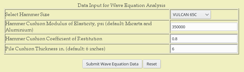


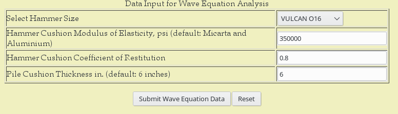

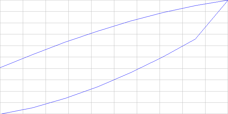
 value computed by
