In this post, we will see the book General Geology by O. Lange; M. Ivanova; N. Lebedeva. About the book The book is a basic introduction to geology. The first two chapters talk about the origin of the Earth and its properties, and the outer geospheres of earth: the atmosphere, hydrosphere, biosphere and lithosphere. The […]
My institution has featured yet another one of my students who graduated last month, Ogheneruona Uwusiaba, from Nigeria.
“Ruona” (as we called her) was a very diligent student, and took all of the classes I taught (Soil Mechanics, Foundations and Fluid Mechanics Laboratory.) To be a student athlete, mother, engineering student and graduate Magna Cum Laude takes a special type of person, and Ruona is that.
This website–and by extension my teaching–goes around the world to the extent that more visits come from outside the U.S. than inside. Sometimes though the world comes to my classroom, and Ruona was a part of that.
Elastic solutions to stresses induced by loads at the surface have their limitations, but they allow the use of the principle of superposition. The principle of superposition states that you can add the effects of different loads on a single point. Superposition requires that the stress state of the point be path independent, which is the case with elastic conditions. No matter how you load and unload a point in a system, if elasticity is maintained the result will be the same for a given set of loads.
This is illustrated for point loads in the graphic below, but it applies to distributed loads (such as this and this) as well.
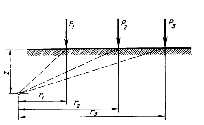
Action of a Number of Concentrated Forces (from Tsytovich (1976))
The stresses that result from each load affect the total stress at the point of interest. They can be computed and added together. So, since “point” loads are physically impossible, is their computation be useful? The answer to this question is “yes” but it takes some judgement, like so many things in geotechnical engineering.
Let us consider the following case, from NAVFAC DM 7.01.
To solve this problem, DM 7 converted the square footings to circular ones and then used the chart shown in the post Going Around in Circles for Rigid and Flexible Foundations. This chart, like others, is hard to read. Is it possible to use point loads as a substitute?
There are three things we need to note here. The first is that the load on each column is 27 tons, and is the same for each column.
The second is that the “r” shown in the table above is not the same as it is for the point loads. The variable “r” for the point loads is the horizontal distance from the load to the point of interest.
The third is that there are three column positions shown in the diagram, with three corresponding values of r:
The column on top of the load, Column B2
The columns in the mid-point of the edges, Columns A2, B1, B3, and C2. These have an value of r of 15′ from the point of interest.
The columns in the corners of the square, Columns A1, A3, C1, and C3. These have a value of r of 21.2′ from the point of interest.
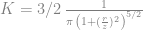
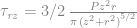
Now, instead of the chart, we apply the formula derived earlier for the influence coefficient, which is
from which the stress is computed by the equation
Using this formula, we can construct the table below for this problem.
(1) Z, ft
(2) r/Z for B2
(3) r/Z for A2, B1, B3, C2
(4) r/z for A1, A3, C1, C3
(5) K for B2
(6) K for A2, B1, B3, C2
(7) K for A1, A3, C1, C3
(8) Stress for B2, tsf
(9) Stress for each of A2, B1, B3, C2, tsf
(10) Stress for each of A1, A3, C1, C3, tst
(11) Total Stress at Z, tsf
2
0
7.500
10.607
0.477
0.000
0.000
3.223
0.000
0.000
3.224
4
0
3.750
5.303
0.477
0.001
0.000
0.806
0.001
0.000
0.810
6
0
2.500
3.536
0.477
0.003
0.001
0.358
0.003
0.001
0.370
10
0
1.500
2.121
0.477
0.025
0.007
0.129
0.007
0.002
0.163
15
0
1.000
1.414
0.477
0.084
0.031
0.057
0.010
0.004
0.113
20
0
0.750
1.061
0.477
0.156
0.073
0.032
0.011
0.005
0.094
25
0
0.600
0.849
0.477
0.221
0.123
0.021
0.010
0.005
0.080
Results from the Separate Column Footings problem in NAVFC DM 7.01, using point loads. Note that the stresses in Columns 9 and 10 are due to a single column, and not all four of them. The total stress in column (11) is the sum of the stress in Column 8 plus 4 times the result in Column 9 plus four times the result in Column 10.
We could have opted to add the influence coefficients and then compute the stresses since, for each elevation Z, both the elevation and the column load were the same. We did not for clarity; it is certainly possible to have columns of different loads.
The results are conservative, they tend to be higher, especially at the lower value elevations. It’s worth noting that the total stress at Z = 2′ is higher than the distributed loads on the footings. One way to make this better is to use the center formulae for stress under circles for Column B2 and point loads for the rest. Given, however, the limitations of the method in general, and the considerably lower effort in obtaining the influence coefficients, the method is a reasonable one to use.
Superposition doesn’t only apply to point loads; the example given in the post Analytical Boussinesq Solutions for Strip, Square and Rectangular Loads uses it for rectangular and square loads. Nevertheless, with appropriate engineering judgement, using point loads in place of distributed loads can be a viable option.
In another post we show the formal, nice way to derive the equations for stresses under point loads. Here we’re going to show a “quick and dirty” way to derive them (or at least some of them.) It’s based on Tsytovich (1976) but I have made some changes to tighten up the theory behind them and make them a little more comprehensible. They don’t derive all of the equations, but the method gives a better physical understanding of what’s going on when we apply such a load to the ground surface.
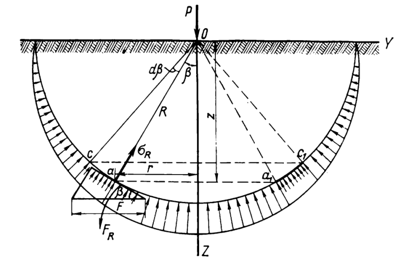
Let’s start with Tsytovich’s diagram, shown below.
Radial stresses under the action of a concentrated force (from Tsytovich (1976))
It can be shown that this state exists due to static equilibrium. The point load P forms a sphere around itself; the principal stresses radiate from the load, forming a sphere around the point of radius R. The magnitude of the stress is given by the equation
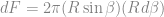
By same static equilibrium, the vertical force of the stresses and P are thus
The infinitesimal surface area of the stress can be defined as
Substituting this into the integral yields
Making appropriate substitutions, the integral evaluates to
and thus
Substituting,
We want the vertical and shear stresses at this point. What we need is a conversion from the polar to cylindrical coordinates, which are given by the equations (Timoshenko and Goodier (1951))
These are coordinate transformations for plane stress equations and are discussed in detail in Boresi et.al. (1993) in terms of the direction cosines of the stress vectors. It may seem odd to see sine terms for these but . If we also assume that , again substituting we have
Since
and
substituting both of these yields our desired result
Many textbooks (such as Verruijt) state these equations in terms of R, but in general problems such as this are defined most simply in terms of the depth of the point of interest z and the horizontal distance from that point r.
For the vertical stresses, if we define an influence coefficient
then
and we can use the following table to determine the influence coefficients K.
Influence Coefficient K to calculate vertical stresses from a concentrated force for a given r/z ratio (from Tsytovich (1976))
The reason we’ve skipped the lateral stresses is because they’re dependent upon the elastic properties of the soil, and also because the vertical stresses are of greater interest.
The point load problem is an important one because many of the area load problems are based on its solution. It can also be used in other ways in spite of the fact that the solution is singular at the point where the load is applied.
Other References
Boresi, A.P., Schmidt, R.J., and Sidebottom, O.M. (1993) Advanced Mechanics of Materials. Fifth Edition. New York: John Wiley and Sons.
Timoshenko, S., and Goodier, J.N. (1951) Theory of Elasticity. New York: McGraww-Hill Book Company, Inc.
In an earlier post Analytical Boussinesq Solutions for Strip, Square and Rectangular Loads, we discussed elastic solutions for these types of foundations. Most of the results shown were for perfectly elastic foundations. In this post we will concentrate on a) circular foundations and b) the difference between rigid and elastic foundations, and those which find themselves in between.
Circular Foundations
Engineers have been familiar with charts such as this, from NAVFAC DM 7.01:
Chart for influence coefficients for uniformly loaded circular foundations, from NAVFAC DM 7.01 (1986). The chart is redrawn from Foster and Ahlvin (1954)
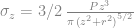
The influence coefficients (see diagram above) for the vertical, horizontal and shear stresses respectively directly under the centre of the load (x = 0) are not difficult to compute, being
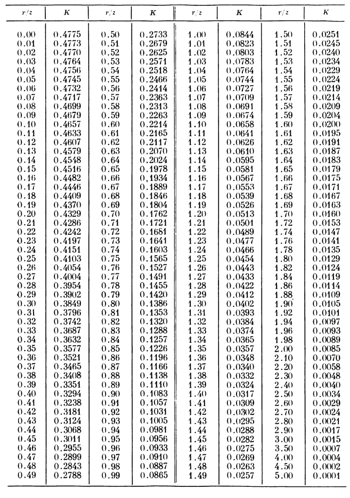
For just about everywhere else (except for the edge) closed form solutions are hard to come by. Why is this? Because, for most every other point, the solution for the influence coefficients involves the use of elliptical integrals. An illustration of the values of these is shown below.
Examples of elliptical integrals (from Jahnke and Emde (1945))
Although mathematical packages such as Maple and Matlab are certainly capable of evaluating these, they are still not the common companions of engineers. Fortunately most of the questions about the stresses under circular foundations centre (sorry!) around the point under x = 0, so the above formulae are useful.
Foundations Rigid and Flexible
Up to this point, we’ve considered for the most part the response of the soil–both stress and deflection–to a purely flexible foundation. For these foundations at the soil-foundation interface the pressure exerted on the foundation and the pressure the foundation exerts on the soil is the same. If there is any rigidity in the foundation–and virtually any foundation has some–then both deflections and stresses in the foundation are redistributed.
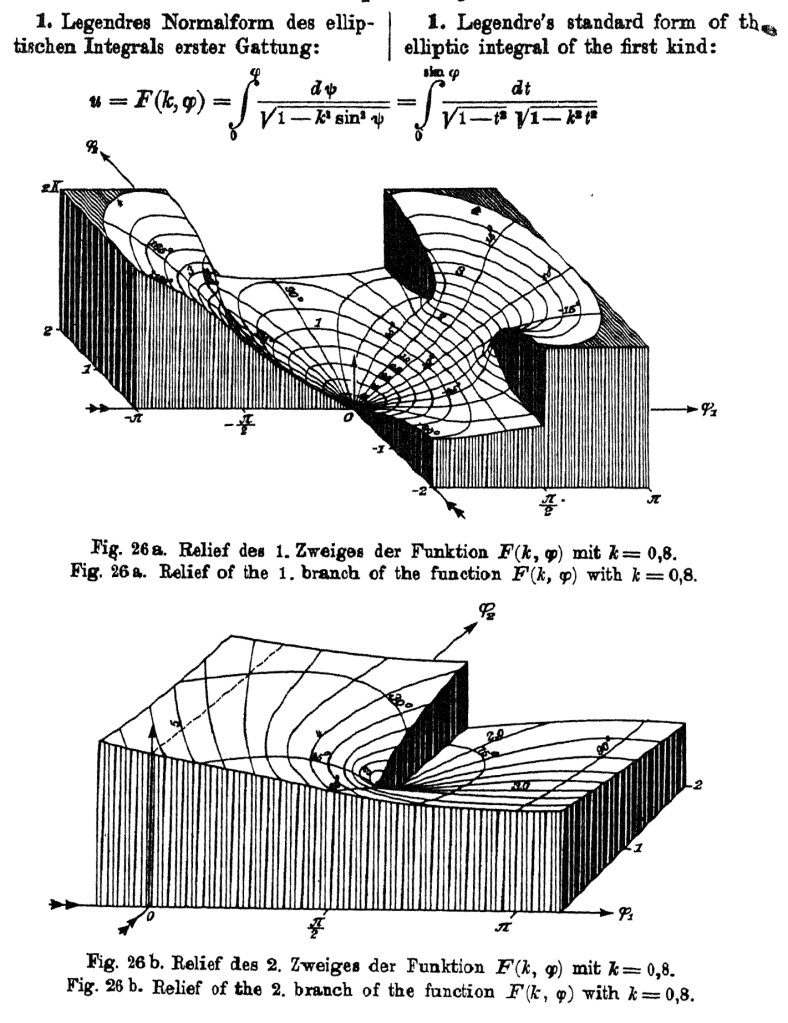
It’s probably useful to note that, for deflections in general, the formula we use is
where
settlement of the foundation at the point of interest
influence factor
uniform pressure on the foundation
smaller dimension of rectangle or dimension of square side
Poisson’s Ratio of the soil
Modulus of elasticity of the soil
The values for are given below.
Values for the influence coefficients omega (from Tsytovich (1976))
Turning to the flexible circular foundation, the value for for all of the radii can be computed using the formula (Timoshenko and Goodier (1951)):
This still has a complete elliptical integral of the second kind, but it more manageable. It can be solved by applying the trapezoidal rule and using small integration increments over the interval. Values for for ratios of various values of x (see diagram above) to the actual radius of the circle are shown below.
x/r
0
1.000
x/r
0.01
1.000
0.51
0.931
0.02
1.000
0.52
0.929
0.03
1.000
0.53
0.926
0.04
1.000
0.54
0.923
0.05
0.999
0.55
0.919
0.06
0.999
0.56
0.916
0.07
0.999
0.57
0.913
0.08
0.998
0.58
0.910
0.09
0.998
0.59
0.906
0.1
0.997
0.6
0.903
0.11
0.997
0.61
0.899
0.12
0.996
0.62
0.896
0.13
0.996
0.63
0.892
0.14
0.995
0.64
0.888
0.15
0.994
0.65
0.884
0.16
0.994
0.66
0.880
0.17
0.993
0.67
0.876
0.18
0.992
0.68
0.872
0.19
0.991
0.69
0.867
0.2
0.990
0.7
0.863
0.21
0.989
0.71
0.859
0.22
0.988
0.72
0.854
0.23
0.987
0.73
0.849
0.24
0.985
0.74
0.844
0.25
0.984
0.75
0.839
0.26
0.983
0.76
0.834
0.27
0.982
0.77
0.829
0.28
0.980
0.78
0.824
0.29
0.979
0.79
0.818
0.3
0.977
0.8
0.813
0.31
0.976
0.81
0.807
0.32
0.974
0.82
0.801
0.33
0.972
0.83
0.795
0.34
0.970
0.84
0.788
0.35
0.969
0.85
0.782
0.36
0.967
0.86
0.775
0.37
0.965
0.87
0.768
0.38
0.963
0.88
0.761
0.39
0.961
0.89
0.754
0.4
0.959
0.9
0.746
0.41
0.957
0.91
0.738
0.42
0.954
0.92
0.730
0.43
0.952
0.93
0.721
0.44
0.950
0.94
0.712
0.45
0.947
0.95
0.702
0.46
0.945
0.96
0.692
0.47
0.942
0.97
0.681
0.48
0.940
0.98
0.669
0.49
0.937
0.99
0.655
0.5
0.934
1
0.637
Values of the influence factor omega vs. the ratio of the radius of a particular point to the entire radius of the circular foundation.
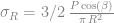
Although many elastic calculations assume the flexible foundation, as noted earlier in reality foundations have rigidity. For a perfectly rigid foundation, the deflection of the entire foundation under a concentric load is uniform. The effect of this on the stresses can be seen below.
Diagrams of contact pressures a) under an absolutely rigid foundation, b) under foundations of various flexibilities. (From Tsytovich (1976))
For the foundation in (a), if it is a circular foundation, the vertical stresses at the base can be computed by the formula
At the corners of the foundation, the stresses are theoretically infinite. This means that the lower bound solution for such a foundation is zero stress. In reality it is reasonable to assume that a) no foundation is perfectly rigid and b) the soil will proceed into plastic deformation, which will redistribute the stresses.
where the notation is as it was in that discussion.
The figure (b) above shows different vertical stress distributions for different flexibility ratios, given by the variable . This can be approximated by the formula (Tsytovich (1976))
The rigidity of the foundation also influences the distribution of stresses under the foundation, as shown below.
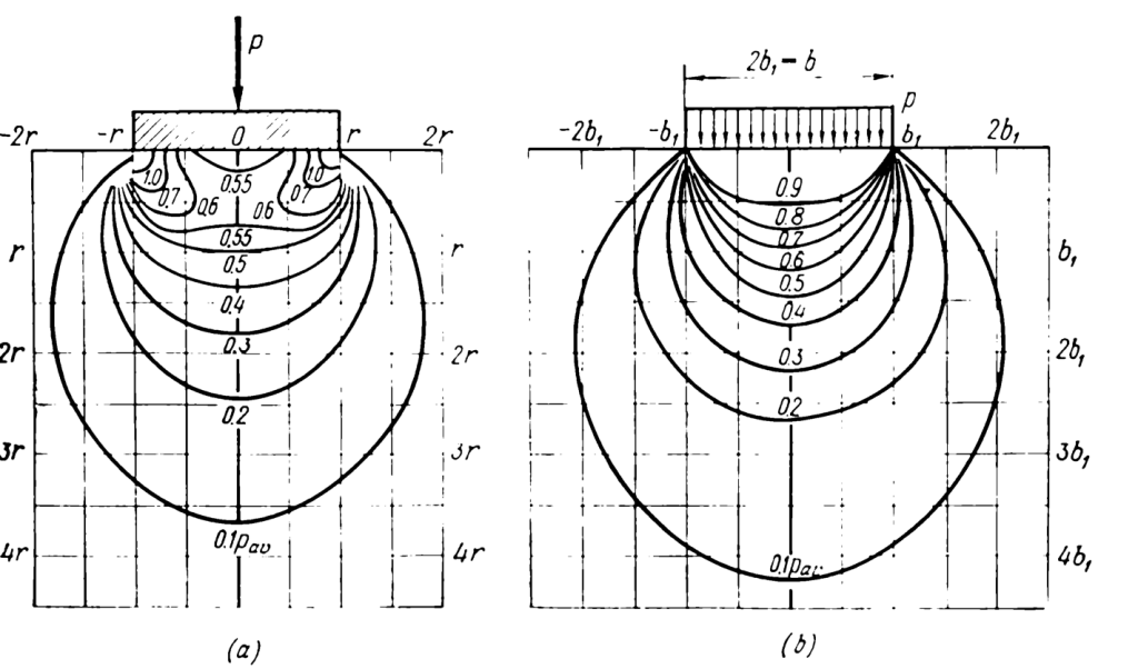
Isobars in Soil under Foundations a)absolutely rigid foundation, b)flexible foundation (from Tsytovich (1976))
There’s certainly life beyond elastic theory. In reality the type of soil affects the distribution of contact pressure on the foundation, even with a uniformly loaded foundation, as shown below.
Contact pressure under a)rigid footings and b)elastic foundation on an elastic half-space (from NAVFAC DM 7.01 (1986))
The clay distribution most resembles that of an elastic response of a soil with a rigid footing, as discussed earlier. The purely flexible foundation will have the same uniform reaction as the load, as noted earlier.
Other Sources
Foster, C.R. and Ahlvin, P.G. (1954) “Stresses and Deflections Induced by Uniform Circular Load.” Highway Research Board Proceedings, Highway Research Board, Washington, DC.
Jahnke, E. and Emde, F. (1945) Tables of Functions with Formulae and Curves. New York: Dover Publishers.
Timoshenko, S., and Goodier, J.N. (1951) Theory of Elasticity. New York: McGraww-Hill Book Company, Inc.


 radiate from the load, forming a sphere around the point of radius R. The magnitude of the stress is given by the equation


 . If we also assume that
  , again substituting we have
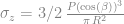


 settlement of the foundation at the point of interest
 influence factor
 uniform pressure on the foundation
 smaller dimension of rectangle or dimension of square side
 Poisson’s Ratio of the soil
 Modulus of elasticity of the soil
 are given below.


 . This can be approximated by the formula (
 modulus of elasticity of the soil
 half-width of the foundation, shown above
 modulus of elasticity of the foundation
 height of the foundation