vulcanhammer.net

An Overview of Mohr-Coulomb Failure Theory

Posted on 16 July 202216 July 2022 by Don Warrington

We now move from elastic considerations to plastic ones. The material that follows is adapted from this dissertation, the development of the STADYN code.

General Remarks About Plasticity

As we transition from elastic to elasto-plastic consideration, there are two things that we need to consider.

The first is that there is more than one way to implement plasticity in finite element and finite difference codes. The one we’ll be considering here–elastic-perfectly plastic behaviour using Mohr-Coulomb failure theory–is just one of them. It appears in many FEA codes, and although is justifiably described as ‘crude’ (Massarsch (1983)) it is the basis (explicit or implicit) of our current testing scheme and many of our ‘closed form’ solutions.

Alternatives not only include models such as Cam Clay but also models such as hyperbolic models. The latter have been discussed extensively on this site and will not be considered further here.

The second is that, because it is plasticity, the response of the soil to load becomes path-dependent. With elastic solutions, the response is path independent; you apply a certain load and the soil responds in a certain way irrespective of how the load is applied. With path dependence how the load is applied affects how the soil responds. This is a large part of another characteristic of plastic solutions: uniqueness issues. As a practical matter true uniqueness, which means a linear transformation which is one-on-one and unto, is impossible. We can only attempt to come up with the best solution. Whether that ‘best solution’ is acceptable depends upon the methodology used and the application. In many cases it is, in some it is not.

Failure Theory

The following is not meant to be a comprehensive treatment of the subject. Much of it is drawn from Nayak and Zienkiewicz (1972) and Owen and Hinton (1980).

According to Mohr-Coulomb theory, failure occurs when the combined stresses find themselves outside of the failure envelope defined by the equation

$\tau=c+\sigma sin\phi$ (1)

This is illustrated in Figure 1.

Figure 1: Mohr-Coulomb Failure Theory (from Tsytovich (1976))

It should be noted that both Equation 1 and Figure 1 are based on the typical geotechnical sign convention of positive compression.

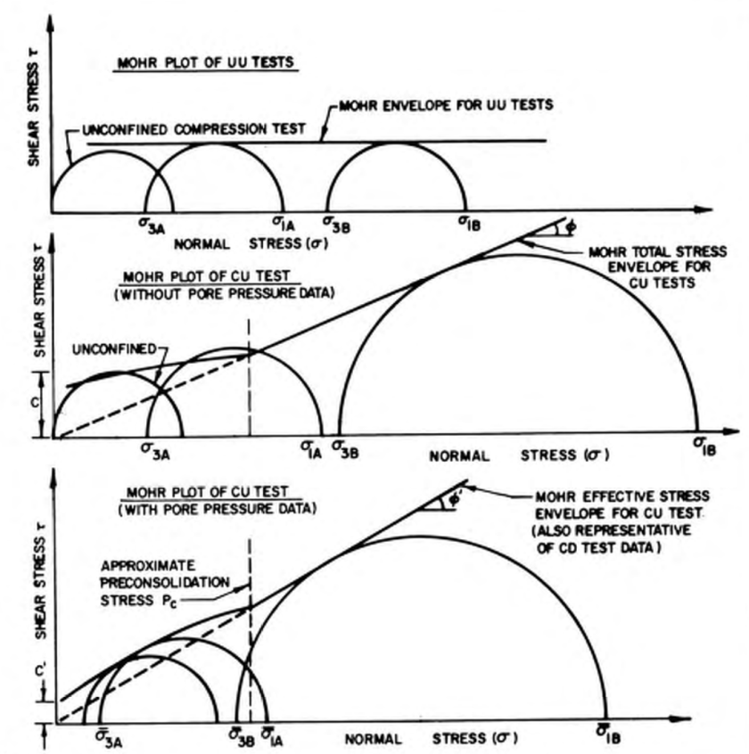
Failure takes place when Mohr’s Circle for the stress state either intersects or goes above the failure line. The state of intersection, in terms of the principal stresses, is expressed by Verruijt as

$\sigma_{1}-\sigma_{{3}}-2c\cos(\phi)+\sin(\phi)\left(\sigma_{{1}}+\sigma_{3}\right)=0$ (2)

For many applications, such as triaxial testing, this is sufficient, as the goal is to determine parameters c and φ from the tests. But what if it is necessary to analyze stress states other than those on the failure line, as is certainly the case with finite elements? For these cases the failure criterion can be defined as

$\sigma_{1}-\sigma_{{3}}-2c\cos(\phi)+\sin(\phi)\left(\sigma_{{1}}+\sigma_{3}\right)=F$ (3)

This is illustrated in Figure 2.

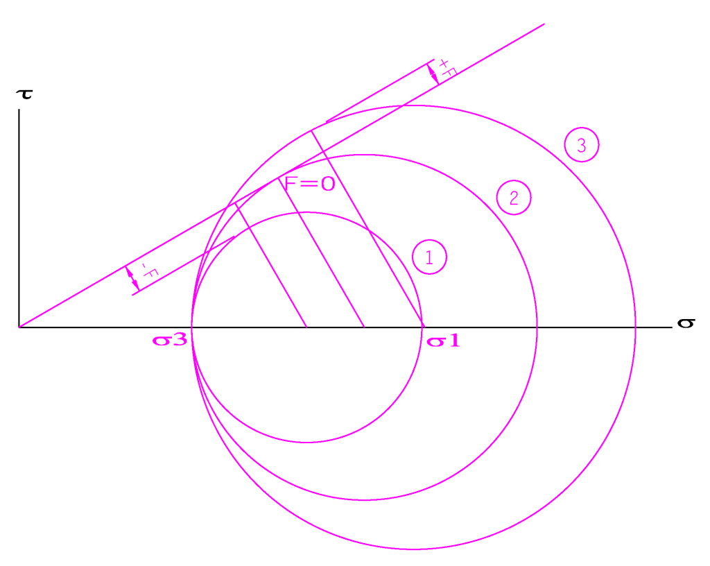
Figure 2: Mohr-Coulomb Failure Criterion (from Warrington (2016))

There are three possibilities for the right hand side:

F<0 , failure has not been achieved.
F=0 , failure has been achieved.
F>0 , the stress state is beyond failure.

How the model responds to each of these states depends upon how the response is modeled. In any case, once F ≥ 0, the effects of further stress are irrecoverable.

For use in finite element code, it is frequently more convenient to express these using invariants. For the case of plane strain/axisymmetry in this problem (and the general case for problems of this kind) it is assumed that

$\tau_{yz}=\tau_{xz}=0$ (4)

and the first invariant is

$J_{1}=\sigma_{x}+\sigma_{y}+\sigma_{z}$ (5)

The deviator stresses are defined as

$\sigma'_{x}=\sigma_{x}-\frac{J_{1}}{3}$
$\sigma'_{y}=\sigma_{y}-\frac{J_{1}}{3}$ (6)
$\sigma'_{z}=\sigma_{z}-\frac{J_{1}}{3}$

The second and third deviatoric invariants are

$J'_{2}=\frac{\sigma{}_{x}^{'2}+\sigma{}_{y}^{'2}+\sigma{}_{z}^{'2}}{2}+\tau_{xy}^{2}$
$J'_{3}=\sigma'_{z}\left(\sigma{}_{z}^{'2}-J'_{2}\right)$ (7)

The whole business of invariants, standard and deviatoric, is discussed in further detail here.

With all of this, Equation 3 can be restated thus:

$\sqrt{J'_{2}}\left(cos\theta-\frac{sin\theta sin\phi}{\sqrt{3}}\right)-c\cos(\phi)+\frac{J_{1}}{3}\sin(\phi)=F$ (8)

where

$\theta=-\frac{1}{3}arcsin\left(\frac{3\sqrt{3}}{2}\frac{J'_{3}}{J_{2}^{'\frac{3}{2}}}\right)$ (9)

The Mohr-Coulomb failure criterion is frequently depicted using a three-dimensional representation on the principal stress axes as is shown (along with the Drucker-Prager criterion) in Figure 3. On the left is the failure surface in true three-dimensional representation, and on the right is same in the octahedral plane. The significance of Lode’s Angle $\theta$ can be clearly seen.

Figure 3: Mohr-Coulomb Failure in Three Dimensions (after Owen and Hinton (1980))

Inspection of Equation 8 shows that the failure function F is not the result of a unique combination of stresses. Additional information is available in the plastic potential function, which in turn is a function of the dilitancy of the material. The simplest way of determining this is by substituting the dilitancy angle ψ for the friction angle φ in Equation 8 (Griffiths and Willson (1986)), or

$\sqrt{J'_{2}}\left(cos\theta-\frac{sin\theta sin\psi}{\sqrt{3}}\right)-c\cos(\psi)+\frac{J_{1}}{3}\sin(\psi)=Q$ (10)

References

Abbo, A.J., Lyamin, A.V., Sloan, S.W., and Hambleton, J.P., “A C2 continuous approximation to the Mohr-Coulomb yield surface”, International Journal of Solids and Structures 48, 21 (2011), pp. 3001–3010.

Gourdin, A. and Boumahrat, M., Méthodes Numériques Appliquées (Paris, France: Téchnique et Documentation-Lavoisier, 1989).

Griffiths, D.V. and Willson, S.M., “An explicit form of the plastic matrix for a Mohr-Coulomb material”, Communications in Applied Numerical Methods 2, 5 (1986), pp. 523–529.

Massarsch, K. Rainer, “Vibration Problems in Soft Soils”, Proceedings of the Symposium on Recent Developments in Laboratory and Field Tests and Analysis of Geotechnical Problems (1983), pp. 539-549.

Nayak, G.C. and Zienkiewicz, O.C., “Elasto/plastic stress analysis. An generalisation for various constitutive relationships.”, International Journal of Numerical Methods in Engineering 5, 1 (1972), pp. 113–135.

Ortiz, M. and Simo, J.C., “An Analysis of a New Class of Integration Algorithms for Elastoplastic Constitutive Relations”, International Journal for Numerical Methods in Engineering 23, 3 (1986), pp. 353–366.

Owen, D.R.J. and Hinton, E., Finite Elements in Plasticity: Theory and Practice (Swansea, Wales: Pineridge Press, 1980).

Potts, D.M. and Zdravković, L., Finite Element Analysis in Geotechnical Engineering: Theory (London, UK: Thomas Telford Publishing, 1999).

Sloan, S.W., “Substepping Schemes for the Numerical Integration of Elastoplastic Stress-Strain Relations”, International Journal for Numerical Methods in Engineering 24, 5 (1987), pp. 893–911.

Verruijt, Arnold and van Baars, S., Soil Mechanics (The Netherlands: VSSD, 2007).

Warrington, Don C., “Application of the STADYN Program to Analyze Piles Driven Into Sand“, vulcanhammer.net (2019).

Nomenclature

$\epsilon$ Strain
$\epsilon^e$ Elastic Strain
$\epsilon^p$ Plastic Strain
$\epsilon_{r,z,rz,\theta}$ Strains in Polar Directions
$\lambda$ Lamé’s Constant, Pa
$\lambda_p$ Elasto-Plastic Normality or Plasticity Constant
$\phi$ Internal Friction Angle, Degrees or Radians
$\psi$ Dilitancy Angle, Degrees or Radians
$\sigma'_{x,y,z}$ Deviator Stress in Cartesian Directions, Pa
$\sigma_{1,3}$ Principal Stresses, Pa
$\sigma_{x,y,z}$ Normal Stressees in Cartesian Directions, Pa
$\tau$ Shear Stress, Pa
$\tau_{xy,yz,xz}$ Shear Stressees in Cartesian Directions, Pa
$\theta$ Lode’s Angle, Radians or Degrees
$a_Q$ Plastic Function Vector
$a_{1,2,3}$ Failure Function Subvectors
$a_{\beta}$ Constant for Substepping Algorithm
$a_F$ Failure Function Vector
$c$ Cohesion, Pa
$C_{1,2,3}$ Failure Function Subconstants
$D^e$ Elastic Constitutive Matrix
$D^p$ Plastic Constitutive Matrix
$D^{ep}$ Elasto-Plastic Constitutive Matrix
$F$ Mohr-Coulomb Failure Criterion, Pa
$G$ Shear Modulus of Elasticity, Pa
$J'_2$ Second Deviatoric Stress Invariant, Pa
$J'_3$ Third Deviatoric Stress Invariant, Pa
$J_1$ First Stress Invariant, Pa
$K_t$ Tangent Stiffness Matrix
$n$ Time or Newton Step Number
$Q$ Plasticity Potential Function, Pa

Geotechnical Engineering

My Thoughts on “DFI’s Rumble: Numerical Modeler vs Skeptic”

Posted on 13 July 2022 by Don Warrington

I found myself interested in the “rumble” between Augusto Lucarelli and Dr. Brian Anderson of Auburn University (not so far from where I teach) about numerical modelling, and the pros and cons of same. For this website, the timing is interesting, coming in the middle of my series on constitutive modelling (there’s more to come, Lord willing.)

You’d think that someone who a) has his terminal degree in Computational Engineering and b) teaches the geotechnical component of the civil engineering undergraduate program at the University of Tennessee at Chattanooga would be an enthusiastic proponent of the use of numerical models for the work. And they’re certainly valuable, but let me just lay out some observations about them in light of the discussion above:

At the start mention was made of using things like SPT tests and Atterberg limits for various determinations. The truth of the matter is that use of lab and field data alike is frequently empirical in its application. If the empirical correlation is not applicable to a certain situation for whatever reason, or the soil data has problems, going from “closed form” (more about that later) solutions to numerical models isn’t going to fix problems of this kind, although it may be better at hiding their deficiencies.
A distinction needs to be made between many of the models we developed in the past and those which are more commonly characterised as “numerical models” now. The USACOE program CBEAR was mentioned (although programs such as CWALSHT, MAGSETII, CSETT, CSANDSET and really Pile Buck’s SPW911 are similar in nature.) These are really computational aids for “closed form” solutions or similar methods. Today a numerical solution is generally finite element or finite difference, such as the COM624/LPILE family, WEAP/GRLWEAP or its inverse CAPWAP, in addition to the numerous finite element codes in use. The former are really automations of things engineers used to do completely by hand; the latter are beyond hand calculation. The advantage of the former is that, although it’s certainly possible to mess up the results with bad input, the possibility of computational error in the process is reduced. With the latter direct replication of the results with hand calculations or closed form solutions is impossible except for very simple cases, and it is here that uncritical acceptance of results is especially dangerous.
It is certainly possible, and desirable during model development, to make a reasonable comparison between a “closed form” solution and one generated by a numerical model provided that the case furnished to the latter is simple enough for reasonable comparison. There are two problems here. The first is that many “modellers” do not make the effort to develop a model in this way by first starting with a simple case and then proceeding to a more complex one. The second is that many of the “closed form” solutions we have in geotechnical engineering are in reality empirical correlations with variable validity. An example of this are the static pile capacity equations, for which there is a proliferation of solutions. This indicates that the science is certainly “not settled,” and in any case runs into the strength vs. service problem (more about that shortly.) The program director for my PhD program said that a good analytical solution was better than a modelled one all other things equal (an example of such a comparison in a simpler case is here.) But finding such a “good analytical solution” in geotechincal engineering isn’t always easy.
I think that the way we’ve taught civil engineering on the undergraduate level does not prepare students for a meaningful understanding of the way finite element and finite difference programs actually work. In some ways it’s more serious than that: the geotechnical component is the first place where students have to face two-dimensional stress distribution in a meaningful way, which has been a major challenge for me teaching these courses over the years. In this respect the way it’s done across the pond (you can see this in texts such as Verruijt and Tsytovich) is better, which may explain some of Dr. Lucarelli’s optimism about this topic. Compounding this problem is the fact that students aren’t required to write code as they used to (Python may change that or may not) which increases the “black box” aspect of packaged models. (In recent years, I find some of my students struggling with engineering spreadsheets…)
Traditionally we’ve divided analytical solutions in geotechnical engineering into three parts: those based on elasticity, those based on plasticity theory and those based on consolidation theory. The advantage of models such as finite element ones is that they can handle more than one of these at a time. The disadvantage is that how these are handled depends upon the model used by the program, something the practicing engineer may or may not understand. For example, those programs which use Mohr-Coulomb theory implemented elasto-plastically use what is admittedly a crude model, but one which fits with a wider range of soils and is better integrated with our current testing scheme. A model used with parameters which have to be “massaged” to fit it is a model asking for trouble.
The entrance of plasticity into models–unavoidable in geotechinical engineering–brings up the whole issue of path dependence, which in turn brings up uniqueness issues for the solution. These are unavoidable; attempts by engineers to produce the single “right” answer are doomed to failure. The happiest result we can hope for is the “best” solution. This pushes things toward a more probabilistic way. Since the advent of LRFD and other statistical methods there is a greater appreciation of this among engineers which may not be shared by clients or those in the legal profession.
The topic of the overemphasis on strength loading (and the corresponding de-emphasis on service loading) is a critical one in geotechnical engineering. Although certain problems (such as slope stability and bearing capacity failure) are catastrophic in nature as they push the soil to the upper bound failure state, most geotechnical problems are with settlement. This is especially true with deep foundations, where service load failure is the greater danger. I know that Bengt Fellenius has beat on this topic for a long time and I attempt to emphasise this with my students as well.
The tendency to throw the solution into the hands of “big data” or “machine learning” without using these tools to sharpen our predictive models is a scientific disaster waiting to happen, and that’s not only true of geotechnical engineering.

I am glad that DFI set this dialogue up, it was informative and timely. I am also glad the Equipment Corporation of America, who was Vulcan Iron Works‘ mid-Atlantic dealer for many years, has sponsored this effort.

Academic Issues

Some Good Advice on Setting Up and Solving Mathematical Problems

Posted on 12 July 2022 by Don Warrington

This, from Computational Mathematics by B. P. Demidovich and I. A. Maron: To illustrate the compilation of a computational scheme, supposeit is …
Some Good Advice on Setting Up and Solving Mathematical Problems

Academic Issues, Geotechnical Engineering

Constitutive Elasticity Equations: Uniaxial Cases

Posted on 11 July 202220 October 2022 by Don Warrington

Our last cases to consider are the cases of uniaxial loading. Although these cases may seem trivial, they are important. As it was with the two-dimensional cases of plane stress and plane strain, there are two variations of the uniaxial loading to consider: uniaxial stress and uniaxial strain.

Uniaxial Stress

We start by considering the constitutive equation of the three-dimensional case, which is

$\left[\begin{array}{cccccc} {\frac{\left(1-\nu\right)\lambda}{\nu}} & \lambda & \lambda & 0 & 0 & 0\\ \noalign{\medskip}\lambda & {\frac{\left(1-\nu\right)\lambda}{\nu}} & \lambda & 0 & 0 & 0\\ \noalign{\medskip}\lambda & \lambda & {\frac{\left(1-\nu\right)\lambda}{\nu}} & 0 & 0 & 0\\ \noalign{\medskip}0 & 0 & 0 & G & 0 & 0\\ \noalign{\medskip}0 & 0 & 0 & 0 & G & 0\\ \noalign{\medskip}0 & 0 & 0 & 0 & 0 & G \end{array}\right]\left[\begin{array}{c} \epsilon_{{x}}\\ \noalign{\medskip}\epsilon_{{y}}\\ \noalign{\medskip}\epsilon_{{z}}\\ \noalign{\medskip}\gamma{}_{{\it xy}}\\ \noalign{\medskip}{\it \gamma}_{{\it yz}}\\ \noalign{\medskip}{\it \gamma}_{{\it zx}} \end{array}\right]=\left[\begin{array}{c} \sigma_{{x}}\\ \noalign{\medskip}\sigma_{{y}}\\ \noalign{\medskip}\sigma_{{z}}\\ \noalign{\medskip}\tau_{{\it xy}}\\ \noalign{\medskip}\tau_{{\it yz}}\\ \noalign{\medskip}\tau_{{\it zx}} \end{array}\right]$ (1)

For uniaxial stress, the following parameters are zero:

$\sigma_y = \sigma_z = 0$ (2a)
$\tau_{xy} = \tau_{xz} = \tau_{yz} = 0$ (2b)

As a result, stress and strain vectors are

$\sigma=\left[\begin{array}{c} \sigma_{{x}}\\ \noalign{\medskip}0\\ \noalign{\medskip}0\\ \noalign{\medskip}0\\ \noalign{\medskip}0\\ \noalign{\medskip}0 \end{array}\right]$ (4)

It’s worth noting that we’ve zeroed out the shear stresses and strains. That’s because, with a uniaxial loading, the x, y and z stresses and strains are guaranteed to be principal stresses and strains, and thus the shear stresses are zero. We will see that the shear stresses and strains will return with axis rotation.

In any case, doing the usual multiplications and inverse multiplications, we have the following:

$\epsilon=\left[\begin{array}{c} \epsilon_{{x}}\\ \noalign{\medskip}\epsilon_{{y}}\\ \noalign{\medskip}\epsilon_{{z}}\\ \noalign{\medskip}0\\ \noalign{\medskip}0\\ \noalign{\medskip}0 \end{array}\right]=\left[\begin{array}{c} -{\frac{\nu\,\sigma_{{x}}}{\lambda\,\left(-1+\nu+2\,{\nu}^{2}\right)}}\\ \noalign{\medskip}{\frac{{\nu}^{2}\sigma_{{x}}}{\lambda\,\left(-1+\nu+2\,{\nu}^{2}\right)}}\\ \noalign{\medskip}{\frac{{\nu}^{2}\sigma_{{x}}}{\lambda\,\left(-1+\nu+2\,{\nu}^{2}\right)}}\\ \noalign{\medskip}0\\ \noalign{\medskip}0\\ \noalign{\medskip}0 \end{array}\right]$ (5)

$\sigma=\left[\begin{array}{c} \sigma_{{x}}\\ \noalign{\medskip}0\\ \noalign{\medskip}0\\ \noalign{\medskip}0\\ \noalign{\medskip}0\\ \noalign{\medskip}0 \end{array}\right]=\left[\begin{array}{c} {\frac{\left(1-\nu\right)\lambda\,\epsilon_{{x}}}{\nu}}+\lambda\,\epsilon_{{y}}+\lambda\,\epsilon_{{z}}\\ \noalign{\medskip}\lambda\,\epsilon_{{x}}+{\frac{\left(1-\nu\right)\lambda\,\epsilon_{{y}}}{\nu}}+\lambda\,\epsilon_{{z}}\\ \noalign{\medskip}\lambda\,\epsilon_{{x}}+\lambda\,\epsilon_{{y}}+{\frac{\left(1-\nu\right)\lambda\,\epsilon_{{z}}}{\nu}}\\ \noalign{\medskip}0\\ \noalign{\medskip}0\\ \noalign{\medskip}0 \end{array}\right]$ (6)

Considering the first rows of Equation (5) gives us

$\epsilon_{{x}}=-{\frac{\nu\,\sigma_{{x}}}{\lambda\,\left(-1+\nu+2\,{\nu}^{2}\right)}}$ (7)

and from the next two rows

$\epsilon_{y}=\epsilon_{z}=-\nu\epsilon_{x}$ (8)

It’s possible to formulate the computation of the stresses based on the strains, but in uniaxial loading it is usually easier to know the stresses first.

Although uniaxial loading is common in tensile and compressive stresses of materials such as metals and plastics, in geotechnical engineering it is mainly concentrated in two types of tests: Triaxial tests and Unconfined Compression (UC) tests. Since in Mohr-Coulomb theory we use a maximum shear stress to determine the point of failure, and the shear stresses and strains don’t appear in the above equations, an explanation as to how shear stresses and strains apply is reasonable.

Rather than go into a math-intensive derivation of the problem, recourse to Mohr’s Circle is more instructive.

Various conditions for triaxial and UC tests (from NAVFAC DM 7.01)

Let’s look at the top diagram from a UC test. The main uniaxial stress $\sigma_1 = \sigma_x$ . If we go 90 degrees anti-clockwise around Mohr’s Circle from $\sigma_1$ , we arrive at the point of maximum shear. This means that the plane of maximum shear is 45 degrees (half Mohr’s Circle angle) from the centre axis of the test specimen. Thus we would expect failure along that plane for a soil that follows Mohr-Coulomb elastic-perfectly plastic behaviour.

In the case of materials with internal friction, things are a little more complicated, because the angle from the principal stress to the point where Mohr’s Circle meets the failure envelope is greater than 90 degrees, thus the angle between the centre axis and the failure plane is greater than 45 degrees, and depends upon the interaction of the cohesion and the internal friction angle.

Of course people who actually run these tests will tell you that these specimens don’t always fail along these planes, or simply bulge at failure. That’s because soils don’t always obey Mohr-Coulomb elastic-perfectly plastic failure theory, which is one of those things that makes geotechnical engineering challenging.

Uniaxial Strain

Although this case doesn’t seem at first glance to be very useful, it’s really an important one for geotechnical engineers. We’ll start again with Equation (1) and zero out the following parameters:

$\epsilon_y = \epsilon_z = 0$ (9)

Of course Equation (2b) applies as well. Doing this results in the following vectors, and I’ll go ahead and multiply and inversely multiply through as before:

$\epsilon=\left[\begin{array}{c} \epsilon_{{x}}\\ \noalign{\medskip}0\\ \noalign{\medskip}0\\ \noalign{\medskip}0\\ \noalign{\medskip}0\\ \noalign{\medskip}0 \end{array}\right]=\left[\begin{array}{c} -{\frac{\nu\,\sigma_{{x}}}{\lambda\,\left(-1+\nu+2\,{\nu}^{2}\right)}}+{\frac{{\nu}^{2}\sigma_{{y}}}{\lambda\,\left(-1+\nu+2\,{\nu}^{2}\right)}}+{\frac{{\nu}^{2}\sigma_{{z}}}{\lambda\,\left(-1+\nu+2\,{\nu}^{2}\right)}}\\ \noalign{\medskip}{\frac{{\nu}^{2}\sigma_{{x}}}{\lambda\,\left(-1+\nu+2\,{\nu}^{2}\right)}}-{\frac{\nu\,\sigma_{{y}}}{\lambda\,\left(-1+\nu+2\,{\nu}^{2}\right)}}+{\frac{{\nu}^{2}\sigma_{{z}}}{\lambda\,\left(-1+\nu+2\,{\nu}^{2}\right)}}\\ \noalign{\medskip}{\frac{{\nu}^{2}\sigma_{{x}}}{\lambda\,\left(-1+\nu+2\,{\nu}^{2}\right)}}+{\frac{{\nu}^{2}\sigma_{{y}}}{\lambda\,\left(-1+\nu+2\,{\nu}^{2}\right)}}-{\frac{\nu\,\sigma_{{z}}}{\lambda\,\left(-1+\nu+2\,{\nu}^{2}\right)}}\\ \noalign{\medskip}0\\ \noalign{\medskip}0\\ \noalign{\medskip}0 \end{array}\right]$ (10)

$\sigma=\left[\begin{array}{c} \sigma_{{x}}\\ \noalign{\medskip}\sigma_{y}\\ \noalign{\medskip}\sigma_{z}\\ \noalign{\medskip}0\\ \noalign{\medskip}0\\ \noalign{\medskip}0 \end{array}\right]=\left[\begin{array}{c} {\frac{\left(1-\nu\right)\lambda\,\epsilon_{{x}}}{\nu}}\\ \noalign{\medskip}\lambda\,\epsilon_{{x}}\\ \noalign{\medskip}\lambda\,\epsilon_{{x}}\\ \noalign{\medskip}0\\ \noalign{\medskip}0\\ \noalign{\medskip}0 \end{array}\right]$ (11)

Extracting the important results,

$\sigma_{{x}}={\frac{\left(1-\nu\right)\lambda\,\epsilon_{{x}}}{\nu}}$ (12)
$\epsilon_{x}={\frac{\sigma_{{x}}\nu}{\left(1-\nu\right)\lambda}}$ (13)
$\sigma_{y}=\sigma_{z}=\frac{\nu}{1-\nu}\sigma_{x}$ (14)

Although it may seem esoteric, this condition is actually important because it simulates confined specimens under uniaxial load. The best known of these, of course, is consolidation testing and all of the variations of that which are employed. It may seem strange to employ elastic theory in this situation, but that speaks to Jean-Louis Briaud’s pet peeve regarding consolidation testing and the partial solution to the problem he poses. Some discussion of this relationship can also be found in Verruijt.

The whole concept of confined specimens is based on the fact that the entire ground upon which we build is a confined specimen, confined by the semi-infinite soil surrounding the loaded portion. Thus this unlikely looking case is very relevant for real geotechnical engineering.

Academic Issues, Geotechnical Engineering

Constitutive Elasticity Equations: Plane Stress

Posted on 9 July 20229 July 2022 by Don Warrington

In our previous posts we discussed three-dimensional and two-dimensional plane strain/axisymmetric constitutive elasticity equations. In this post we will consider plane stress. This case doesn’t appear very much in geotechnical engineering; it’s more of interest to mechanical engineers and deals with problems such as this.

It’s probably a good idea to look again at the graphic for this:

Plane stress, plane strain and axial symmetry cases, from Owen and Hinton (1980)

The conditions of plane stress are thus:

$\sigma_z = 0$ (1a)
$\tau_{xz} = 0$ (1b)
$\tau_{yz} = 0$ (1c)

If we compare these to plane strain, we find out that we switch the z-strain for the z-stress. This means that deriving the equations–especially the 3 x 3 case–is the mirror image of the plane strain case, and we will see this clearly below.

Let’s start by noting that, as before, the starting 4 x 4 constitutive matrix is the same as plane strain, thus

$D_{e}=\left[\begin{array}{cccc} {\frac{\left(1-\nu\right)\lambda}{\nu}} & \lambda & \lambda & 0\\ \noalign{\medskip}\lambda & {\frac{\left(1-\nu\right)\lambda}{\nu}} & \lambda & 0\\ \noalign{\medskip}\lambda & \lambda & {\frac{\left(1-\nu\right)\lambda}{\nu}} & 0\\ \noalign{\medskip}0 & 0 & 0 & G \end{array}\right]$ (2)

and its inverse

$D_{e}^{-1}=\left[\begin{array}{cccc} -{\frac{\nu}{\lambda\,\left(-1+\nu+2\,{\nu}^{2}\right)}} & {\frac{{\nu}^{2}}{\lambda\,\left(-1+\nu+2\,{\nu}^{2}\right)}} & {\frac{{\nu}^{2}}{\lambda\,\left(-1+\nu+2\,{\nu}^{2}\right)}} & 0\\ \noalign{\medskip}{\frac{{\nu}^{2}}{\lambda\,\left(-1+\nu+2\,{\nu}^{2}\right)}} & -{\frac{\nu}{\lambda\,\left(-1+\nu+2\,{\nu}^{2}\right)}} & {\frac{{\nu}^{2}}{\lambda\,\left(-1+\nu+2\,{\nu}^{2}\right)}} & 0\\ \noalign{\medskip}{\frac{{\nu}^{2}}{\lambda\,\left(-1+\nu+2\,{\nu}^{2}\right)}} & {\frac{{\nu}^{2}}{\lambda\,\left(-1+\nu+2\,{\nu}^{2}\right)}} & -{\frac{\nu}{\lambda\,\left(-1+\nu+2\,{\nu}^{2}\right)}} & 0\\ \noalign{\medskip}0 & 0 & 0 & {G}^{-1} \end{array}\right]$ (3)

The stress and strain vectors, however, are

$\sigma=\left[\begin{array}{c} \sigma_{{x}}\\ \noalign{\medskip}\sigma_{{y}}\\ \noalign{\medskip}0\\ \noalign{\medskip}\tau_{{\it xy}} \end{array}\right]$ (4)

$\epsilon=\left[\begin{array}{c} \epsilon_{{x}}\\ \noalign{\medskip}\epsilon_{{y}}\\ \noalign{\medskip}\epsilon_{z}\\ \noalign{\medskip}{\it \gamma}_{{\it xy}} \end{array}\right]$ (5)

We see Equation (1a) applied to the stress vector to yield Equation (4). Multiplying through as we did before,

$\sigma=\left[\begin{array}{c} \sigma_{{x}}\\ \noalign{\medskip}\sigma_{{y}}\\ \noalign{\medskip}0\\ \noalign{\medskip}\tau_{{\it xy}} \end{array}\right]=\left[\begin{array}{c} {\frac{\left(1-\nu\right)\lambda\,\epsilon_{{x}}}{\nu}}+\lambda\,\epsilon_{{y}}+\lambda\,\epsilon_{{z}}\\ \noalign{\medskip}\lambda\,\epsilon_{{x}}+{\frac{\left(1-\nu\right)\lambda\,\epsilon_{{y}}}{\nu}}+\lambda\,\epsilon_{{z}}\\ \noalign{\medskip}\lambda\,\epsilon_{{x}}+\lambda\,\epsilon_{{y}}+{\frac{\left(1-\nu\right)\lambda\,\epsilon_{{z}}}{\nu}}\\ \noalign{\medskip}G{\it \gamma}_{xy} \end{array}\right]$ (6)

$\epsilon=\left[\begin{array}{c} \epsilon_{{x}}\\ \noalign{\medskip}\epsilon_{{y}}\\ \noalign{\medskip}\epsilon_{z}\\ \noalign{\medskip}{\it \gamma}_{{\it xy}} \end{array}\right]=\left[\begin{array}{c} -{\frac{\nu\,\sigma_{{x}}}{\lambda\,\left(-1+\nu+2\,{\nu}^{2}\right)}}+{\frac{{\nu}^{2}\sigma_{{y}}}{\lambda\,\left(-1+\nu+2\,{\nu}^{2}\right)}}\\ \noalign{\medskip}{\frac{{\nu}^{2}\sigma_{{x}}}{\lambda\,\left(-1+\nu+2\,{\nu}^{2}\right)}}-{\frac{\nu\,\sigma_{{y}}}{\lambda\,\left(-1+\nu+2\,{\nu}^{2}\right)}}\\ \noalign{\medskip}{\frac{{\nu}^{2}\sigma_{{x}}}{\lambda\,\left(-1+\nu+2\,{\nu}^{2}\right)}}+{\frac{{\nu}^{2}\sigma_{{y}}}{\lambda\,\left(-1+\nu+2\,{\nu}^{2}\right)}}\\ \noalign{\medskip}{\frac{\tau_{{\it xy}}}{G}} \end{array}\right]$ (7)

If we equation the two third row elements of the vectors in Equation (6), we have

$\lambda\,\epsilon_{{x}}+\lambda\,\epsilon_{{y}}+{\frac{\left(1-\nu\right)\lambda\,\epsilon_{{z}}}{\nu}}=0$ (8)

Solving for the z-axis strain,

$\epsilon_{z}={\frac{\left(\epsilon_{{x}}+\epsilon_{{y}}\right)\nu}{-1+\nu}}$ (9)

Since the z-axis strain is a function of the x-axis and y-axis strains, the obvious question is this: can we go to a 3 x 3 matrix formulation? The answer is yes if we literally invert the process. We need to do the following:

Consider the basic equation in this form: $D_{e}^{-1}\sigma=\epsilon$ .
Since $\sigma_z = 0$ , we can remove the third column and row from the constitutive matrix and the third row from the stress (and strain) matrix.
We multiply through to yield

$\left[\begin{array}{ccc} -{\frac{\nu}{\lambda\,\left(-1+\nu+2\,{\nu}^{2}\right)}} & {\frac{{\nu}^{2}}{\lambda\,\left(-1+\nu+2\,{\nu}^{2}\right)}} & 0\\ \noalign{\medskip}{\frac{{\nu}^{2}}{\lambda\,\left(-1+\nu+2\,{\nu}^{2}\right)}} & -{\frac{\nu}{\lambda\,\left(-1+\nu+2\,{\nu}^{2}\right)}} & 0\\ \noalign{\medskip}0 & 0 & {G}^{-1} \end{array}\right]\left[\begin{array}{c} \sigma_{{x}}\\ \noalign{\medskip}\sigma_{{y}}\\ \noalign{\medskip}\tau_{{\it xy}} \end{array}\right]=\left[\begin{array}{c} \epsilon_{{x}}\\ \noalign{\medskip}\epsilon_{{y}}\\ \noalign{\medskip}{\it \gamma}_{{\it xy}} \end{array}\right]=\left[\begin{array}{c} -{\frac{\nu\,\sigma_{{x}}}{\lambda\,\left(-1+\nu+2\,{\nu}^{2}\right)}}+{\frac{{\nu}^{2}\sigma_{{y}}}{\lambda\,\left(-1+\nu+2\,{\nu}^{2}\right)}}\\ \noalign{\medskip}{\frac{{\nu}^{2}\sigma_{{x}}}{\lambda\,\left(-1+\nu+2\,{\nu}^{2}\right)}}-{\frac{\nu\,\sigma_{{y}}}{\lambda\,\left(-1+\nu+2\,{\nu}^{2}\right)}}\\ \noalign{\medskip}{\frac{\tau_{{\it xy}}}{G}} \end{array}\right]$ (10)

We then invert the inverse to obtain the 3 x 3 constitutive matrix. We use the forward formulation $D\epsilon=\sigma$ and multiply through to obtain

$\left[\begin{array}{ccc} {\frac{\lambda\,\left(-1+2\,\nu\right)}{\nu\,\left(-1+\nu\right)}} & {\frac{\lambda\,\left(-1+2\,\nu\right)}{-1+\nu}} & 0\\ \noalign{\medskip}{\frac{\lambda\,\left(-1+2\,\nu\right)}{-1+\nu}} & {\frac{\lambda\,\left(-1+2\,\nu\right)}{\nu\,\left(-1+\nu\right)}} & 0\\ \noalign{\medskip}0 & 0 & G \end{array}\right]\left[\begin{array}{c} \epsilon_{{x}}\\ \noalign{\medskip}\epsilon_{{y}}\\ \noalign{\medskip}{\it \gamma}_{{\it xy}} \end{array}\right]=\left[\begin{array}{c} \sigma_{{x}}\\ \noalign{\medskip}\sigma_{{y}}\\ \noalign{\medskip}\tau_{{\it xy}} \end{array}\right]=\left[\begin{array}{c} {\frac{\lambda\,\left(-1+2\,\nu\right)\epsilon_{{x}}}{\nu\,\left(-1+\nu\right)}}+{\frac{\lambda\,\left(-1+2\,\nu\right)\epsilon_{{y}}}{-1+\nu}}\\ \noalign{\medskip}{\frac{\lambda\,\left(-1+2\,\nu\right)\epsilon_{{x}}}{-1+\nu}}+{\frac{\lambda\,\left(-1+2\,\nu\right)\epsilon_{{y}}}{\nu\,\left(-1+\nu\right)}}\\ \noalign{\medskip}G{\it \gamma}_{{\it xy}} \end{array}\right]$ (11)