Uncategorized – vulcanhammer.net

NAVFAC DM 7.2: Earthwork, Hydraulic and Underwater

Posted on 17 April 2025 by Don Warrington

The whole topic of earthwork and compaction is one whose coverage is inconsistent, to say the least, in basic geotechnical publications. Some do a very good job, others ignore it altogether. NAVFAC DM 7.2 has done a very thorough job on the subject, covering topics which are scarce in other places. Compaction is the oldest earth improvement technique we have and is still the most commonly used on construction sites around the world.

There are many topics which are explored in this chapter; I will only mention a few of them. It’s hard to distill all of the information in the book; you’ll just have to get it and find out for yourself. Some of them (such as compaction equipment types and sample fill specifications) are carried over and expanded from the previous document; others are new.

Line of Optimums Method

When I was first brought on board to Soils in Construction, I learned about this, which I discuss in this post (illustration of the method is at the right.) There were few references on the subject to be found, which made Soils in Construction somewhat unique. (I need to say kudos to my co-author, Lee Schroeder, especially for the part of the book on compaction.) We actually got thumbs up during the review process for including it. This edition of NAVFAC DM 7.2 has fixed that lacuna with a section on the subject. I don’t see how one can actually specify a compaction method without it, especially if experience is lacking and/or the soils are variable on a site. They have included information on the effects of “dry of optimum” (left of line 6 on the chart above) and “wet of optimum (right of line 6) as well. All in all, a very nice treatment on the subject.

Making the Cut with Borrow and Fill Calculations

Another topic covered in Soils in Construction is that of borrow and fill calculations. Some soil mechanics books cover this, some don’t. It’s covered in detail in NAVFAC DM 7.2. It will definitely help you to “make the cut” when excavating, transporting, placing and compacting fill materials.

Hydraulic Fills

Many geotechical references treat hydraulic fills as a thing of the past after some early disasters involving them. Evidently not; there is a whole chapter on the subject, both for understanding dams built in this way and for underwater fills, when hydraulic fills are virtually unavoidable.

Uncategorized

Analysing a Gravity Wall Using Vector Analysis

Posted on 6 January 2025 by Don Warrington

One of the reasons I was interested in teaching Statics at Lee University was because I was continually disappointed at my students’ memory of their statics. Statics is crucial in the design and analysis of geotechnical structures, and most of the problems–at the undergraduate level at least–aren’t that involved, or at least I thought they weren’t. A great deal of the problem is that geotechnical statics usually involves converting distributed loads into resultants, which Statics–and Mechanics of Materials for that matter–generally associate this with beam problems, not always the case with geotechnical problems.

Another culprit is that Statics, in the U.S. at least, is a vector proposition from the start. At the University of Tennessee at Chattanooga where I taught, it was called “Vector Statics,” which gives the game away early. (At Lee we use the same book and teach the same material, but simply title it “Statics.”)

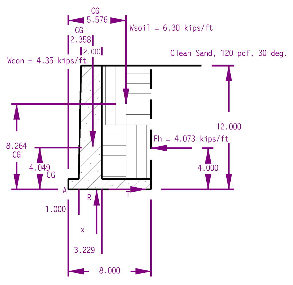
But what if we applied a vector approach to a simple geotechnical problem? That’s what we’re going to do here with a concrete gravity wall. I will use the method outlined in my post A Simplified Method to Design Cantilever Gravity Walls. You can refer to the theory there, I will try to keep it to a minimum. The wall is pictured at the top of the post, I will reproduce it below.

Analysing Overturning

We have three forces acting on the wall:

The weight of the gravity wall itself, W_conc
The weight of the soil trapped by the heel of the wall, W_soil
The lateral force of the soil on the wall, F_h

Forces 1 and 2 are determined by computing the cross-sectional area of the concrete and soil and multiplying each by the unit weight as shown above, and then converting the result to a vector force and placing it at the centroid of the area (another Statics topic.) Instead of the “manual” approach in A Simplified Method to Design Cantilever Gravity Walls, the was was drawn in CAD and both the areas and centroids were determined automatically. You can see the magnitudes and locations of those resultants above.

The lateral force of the soil is computed using Rankine’s theory. The first thing is to determine the working internal friction angle of the soil by applying the Shear Mobilisation Factor SMF. Assuming an SMF of 2/3, that friction angle changes from the 30 degree one shown above to a 21.05 degree one, which is applied to the formula for Rankine active pressures for level backfill,

$k_h = \frac{1-sin\phi}{1+sin\phi}$ (1)

Doing that results in a k_h = .471. The force on the wall is then determined by the formula

$F_h = \frac{k_h\gamma_{soil}H^2}{2}$ (2)

The division by two reflects the fact that soil effective stress (and thus lateral earth pressure) increases linearly with depth (like a fluid,) creating a triangular distribution (yet another concept from Statics.)

At this point there the resisting forces R and T are not defined. The forces themselves are easily computed by summing forces in the x and y directions. Doing this, we have

$R = -W_{conc}-W_{soil}$ (3a)
$T = -F_{h}$ (3b)

The location of F–along the surface of the footing–is evident. The location of R is not; it is some distance x from the toe (Point “A”) of the footing. We can obtain x by summing moments around Point “A,” and with a vector method that means taking cross products of the moment arms with the forces.

Converting both the moment arms r and the forces to vector notation yields the following:

Concrete Weight: r = 2.358 i + 4.049 j, W_con = −4.35 j
Soil Weight: r = 5.576 i + 8.264 j, W_soil = −6.30 j
Lateral Earth Pressure: r = 8 i + 4 j, F_h = −4.073261616 i
Vertical Footing Force: r = x i, R = 10.65 j (Equation (3a))

The force T does not enter into this because its line of action runs through Point “A,” thus its moment is zero as its moment arm is zero.

The cross product moments around the toe (Point “A” in the drawing) are as follows:

Concrete Weight: $\left [\begin {array}{ccc} i&j&k\\{\medskip} 2.358& 4.049&0 \\{\medskip}0&- 4.35&0\end {array}\right ] = -10.257 k$
Soil Weight: $\left [\begin {array}{ccc} i&j&k\\{\medskip} 5.576& 8.264&0\\{\medskip}0&- 6.3&0\end {array}\right ] = -35.129k$
Lateral Earth Pressure: $\left [\begin {array}{ccc} i&j&k\\{\medskip}8&4&0\\{\medskip}- 4.073&0&0\end {array}\right ] = 16.293k$
Vertical Footing Force: $\left [\begin {array}{ccc} i&j&k\\{\medskip}x&0&0\\{\medskip}0& 10.65&0\end {array}\right ] = 10.65 x k$

Summing these moments,

$29.093\,k+ 10.65\,xk=0$ (4)

Solving yields x = 2.732′. At this point we need to determine whether this is an acceptable location or not for the force. The goal is for the pressure to be positive (downward) along the entire surface of the footing. There are two ways of determining this:

Computing the pressures on each end of the footing, as is done in A Simplified Method to Design Cantilever Gravity Walls.
Determining whether the force is in the “middle third” of the foundation, as is discussed in the Soils and Foundations Reference Manual.

We will do the latter. The middle third of this foundation falls between 2.67′ < x < 5.33′, so the vertical footing force is within the middle third (barely.) As I noted in A Simplified Method to Design Cantilever Gravity Walls, “In this case we make a common assumption that, as long as the resultant force of the wall is within the kern and there are no negative pressures on the base, overturning will not be experienced. It is certainly possible to do an explicit overturning analysis to check this result.”

Analysing Sliding

With the lack of keys or deep foundations, the only lateral resistance to sliding is the friction force T. We computed that force based on Equation (3b,) but in reality that force cannot exceed–and there should be a factor of safety in that inequality–the frictional force possible, which is defined by the equation

$T_{max} = \mu R$ (5)

in which case

$FS_{Sliding} = \frac{T_{max}}{T}$ (6)

Equation (5) is written in “mechanical engineers format.” Geotechnical engineers understand all too well the concept of a friction angle. In my post Explaining the Relationship Between the Coefficient and the Angle of Friction I relate the two from a non-geotech standpoint; we can turn Equation (5) into a more “geotech-friendly” form by noting that

$\mu = \tan\phi$ (7)

Let us assume that the value of $\phi$ is the same under the wall as next to the wall, and let us also assume that the friction angle between the base and the soil is the same as the friction angle of the soil overall, as was done in A Simplified Method to Design Cantilever Gravity Walls. That being the case, $\mu = \tan(30) = 0.577$ . Substituting into Equation (5,) $T_{max} = 0.577 \times 10.65 = 6.15\,kips$ . The factor of safety from Equation (6) is thus $FS_{Sliding} = \frac{6.15}{4.073} = 1.51$ , which is barely over the minimum criterion for usual loads given in A Simplified Method to Design Cantilever Gravity Walls.

Observations

The use of vectors for this problem is overkill from a computational standpoint. It also requires locating the centroid/CG of the two regions in both the x- and y-directions, although with using CAD this is trivial. On the other hand doing it using vectors is more “bullet proof” in that the student is not required to “think” but just “plug and chug” without having to identify lines of action and perpendicular moment arms.
The fact that the word “barely” appears in both analyses should inspire some additional conservatism in the design. The simplest way to improve the situation would be to move the heel to the right, which would shift the resisting forces away from the toe (and thus increase their resisting moment) and also put the footing force resultant deeper into the middle third.
Both bearing capacity and settlement of the wall’s foundation, the methodology for which are discussed in A Simplified Method to Design Cantilever Gravity Walls, are beyond the scope of this post. Also beyond the scope of this post is the structural design of the wall and of course the global stability of the wall as well.

Uncategorized

NAVFAC DM 7.1 Gets 2022 Refresh — GeoPrac.net

Posted on 30 September 202230 September 2022 by Don Warrington

Nearly every geotechnical engineer has referred to the venerable 1986 NAVFAC DM 7.1 Manual on Soil Mechanics. There are numerous useful charts, correlations, tables, and equations for a variety of geotechnical challenges, which is probably […]
NAVFAC DM 7.1 Gets 2022 Refresh — GeoPrac.net

That didn’t take long…after our post The “Before and After” of NAVFAC DM 7, I was made aware of this. This has been posted to our Soil Mechanics page. As far as a print version is concerned, we are considering this, the old version continues to be available.

Uncategorized

Elasto-Perfect Plasticity with Mohr-Coulomb Failure

Posted on 16 July 20223 June 2023 by Don Warrington

This is a continuation of the previous post on Mohr-Coulomb Failure. The references and nomenclature there apply to this post as well.

With the Mohr-Coulomb failure criterion defined, the elasto-plastic constitutive matrix can be developed. Since pure plasticity is assumed, thus once failure is reached and F=0 , the stresses can “rearrange” themselves to remain at the failure surface but cannot move from it unless the strains are reduced to the point where the stress state is within the failure surface and F<0. This is easier to see if we look at the diagram above. We should also note that, for this presentation, the plane strain/axisymmetric case will be considered; the derivation would proceed a little differently for other cases such as plane stress or three-dimensional stress.

To do this, both Equations 8 and 10 from the previous post are differentiated. Considering that

$\sigma=\left[\begin{array}{c} \sigma_{x}\\ \sigma_{y}\\ \sigma_{z}\\ \tau_{xy} \end{array}\right]$ (1)

for the two-dimensional model, then

$\frac{\partial F}{\partial\sigma}=a_{F}=C_{1}a_{1}+C_{2}a_{2}+C_{3}a_{3}$ (2)

where

$C_{1}=\frac{sin\phi}{3}$
$C_{2}=cos\theta\left[\left(1+tan\theta tan3\theta\right)+\frac{sin\phi\left(tan3\theta-tan\theta\right)}{\sqrt{3}}\right]$ (3)
$C_{3}=\frac{\sqrt{3}sin\theta+cos\theta sin\phi}{2J'_{2}cos3\theta}$

and

$a_{1}=\left[\begin{array}{c} 1\\ 1\\ 1\\ 0 \end{array}\right]$
$a_{2}=\frac{1}{2\sqrt{J'_{2}}}\left[\begin{array}{c} \sigma'_{x}\\ \sigma'_{y}\\ \sigma'_{z}\\ 2\tau_{xy} \end{array}\right]$ (4)
$a_{3}=\left[\begin{array}{c} \sigma'_{y}\sigma'_{z}+\frac{J'_{2}}{3}\\ \sigma'_{x}\sigma'_{z}+\frac{J'_{2}}{3}\\ \sigma'_{y}\sigma'_{x}-\tau_{xy}^{2}+\frac{J'_{2}}{3}\\ -2\sigma'_{z}\tau_{xy} \end{array}\right]$

Inspection of Equation 3 will show that C₂ and C₃ are undefined for values of θ =30°. This is the well known “corner” problem which has occupied the literature for many years, as summarized by Abbo et.al. (2011). For this study the “corner cutting” of Owen and Hinton (1980) is used, and

$C_{1}=\frac{sin\phi}{3}$
$C_{2}=\frac{1}{2}\left[\sqrt{3}-\frac{sin\phi}{\sqrt{3}}\right],\:\theta\approx\pm30^{\circ}$ (5)
$C_{3}=0$

Although the accuracy of this “corner cutting” can be improved with methods such as those of Abbo et.al. (2011), they come at more computational expense.

In like fashion for the plastic potential function,

$\frac{\partial Q}{\partial\sigma}=a_{Q}=C_{4}a_{1}+C_{5}a_{2}+C_{6}a_{3}$ (6)

where

$C_{4}=\frac{sin\psi}{3}\\C_{5}=cos\theta\left[\left(1+tan\theta tan3\theta\right)+\frac{sin\psi\left(tan3\theta-tan\theta\right)}{\sqrt{3}}\right]\\C_{6}=\frac{\sqrt{3}sin\theta+cos\theta sin\psi}{2J'_{2}cos3\theta}$ (7)

and by extension

$C_{4}=\frac{sin\psi}{3}\\C_{5}=\frac{1}{2}\left[\sqrt{3}-\frac{sin\psi}{\sqrt{3}}\right],\:\theta\approx\pm30^{\circ}\\C_{6}=0$ (8)

and the vectors a₁ , a₂ , a₃ are the same as with Equation 2.

At this point we need to pause and consider how we plan to present our result. It’s certain possible, for example, to multiply through Equations 2, 3, and 4 and use this result in subsequent derivations. This approach suffers from two problems: the element expressions in the matrices and vectors become very complicated, and the computation cost is increased by the repetitive calculations. For some good advice on this subject–for this and other problems–we would suggest that you review this.

Now the elasto-plastic constitutive matrix can be considered. Here the difference between path indepedence and path dependence becomes significant. In the elastic case, we can use the elastic consitutive matrix D^e and, knowing the strains, compute the stresses, and perform the inverse as well. With plasticity, it is necessary to compute the strains and stresses incrementally, moving from one stress and strain state to the next and adding the results to what has gone before. We do this with both elastic, plastic and combined strains and stresses for computational consistency. The elastic results will be the same except for the additional accumulation of numerical error due to the larger number of computations.

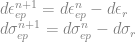
For any strain increment partially or totally beyond the yield surface, that strain increment will contain both elastic and plastic portions (Griffiths and Willson (1986)), or

$d\epsilon=d\epsilon^{e}+d\epsilon^{p}$ (9)

Strain increments occur normal to the plastic potential surface, thus

$d\epsilon^{p}=\lambda_{p}a_{Q}$ (10)

For elastic materials, the incremental stress-strain relationship is simply

$d\sigma=D^{e}d\epsilon^{e}$ (11)

where, for plane strain and axisymmetric problems, as before,

$D^{e}=\left[\begin{array}{cccc} {\frac{\left(1-\nu\right)\lambda}{\nu}} & \lambda & \lambda & 0\\ \noalign{\medskip}\lambda & {\frac{\left(1-\nu\right)\lambda}{\nu}} & \lambda & 0\\ \noalign{\medskip}\lambda & \lambda & {\frac{\left(1-\nu\right)\lambda}{\nu}} & 0\\ \noalign{\medskip}0 & 0 & 0 & G \end{array}\right]$ (12)

and also, for axisymmetric problems only,

$\epsilon^{e}=\left[\begin{array}{c} \epsilon_{r}\\ \epsilon_{z}\\ \epsilon_{\theta}\\ \epsilon_{rz} \end{array}\right]$ (13)

For a perfectly elasto-plastic material, i.e., one without hardening or softening, stress changes will take place only during elastic action. Thus in these cases Equations 9, 10 and 11 can be rearranged to yield

$d\sigma=D^{e}\left(d\epsilon-\lambda_{p}a_{Q}\right)$ (14)

Since stresses on the failure surface can “rearrange” themselves without leaving same surface,

$a_{F}^{t}d\sigma=0$ (15)

Combining and rearranging Equations 9 through 15 yields the following relationships:

$\lambda_{p}=\frac{a_{F}^{t}D^{e}d\epsilon}{a_{F}^{t}D^{e}a_{Q}}$ (16)

$d\sigma=\left(D^{e}-\frac{D^{e}a_{Q}a_{F}^{t}D^{e}}{a_{F}^{t}D^{e}a_{Q}}\right)d\epsilon$ (17)

$d\sigma=\left(D^{e}-D^{p}\right)d\epsilon$ (18)

where

$D^{p}=\frac{D^{e}a_{Q}a_{F}^{t}D^{e}}{a_{F}^{t}D^{e}a_{Q}}$ (19)

and finally

$D^{ep}=D^{e}-D^{p}$ (20)

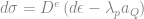
We need to break this down for greater understanding. Let us first define

$a_{\beta}=\frac{1}{a_{F}^{t}D^{e}a_{Q}}$ (21)

This is a scalar quantity. (Admittedly sometimes it is difficult to follow matrix equations because they combine scalar and vector/matrix quantities.) We can thus rewrite Equation 19

$D^{p}=a_{\beta}\left(D^{e}a_{Q}a_{F}^{t}\right)D^{e}$ (22)

and Equation 20 can be likewise rewritten as

$D^{ep}=\left(I-a_{\beta}\left(D^{e}a_{Q}a_{F}^{t}\right)\right)D^{e}$ (23)

where $I =$ the identity matrix.

If plasticity has not yet been initiated, the quantity $a_{\beta}\left(D^{e}a_{Q}a_{F}^{t}\right)$ (which is a 4 x 4 matrix) is null, and the elasticity matrix governs. Once it is initiated the magnitude of $a_{\beta}\left(D^{e}a_{Q}a_{F}^{t}\right)$ begins to increase and D^ep begins to decrease, which indicates a ‘softening’ of the material. This is what we would expect with plasticity. The whole topic of matrix magnitude is not a straightforward one and is usually viewed in relationship to matrix norms, which are discussed in Gourdin and Boumharat (1989).

In any case

$d\sigma=D^{ep}d\epsilon=\left(D^{e}-D^{p}\right)d\epsilon=\left(I-a_{\beta}\left(D^{e}a_{Q}a_{F}^{t}\right)\right)D^{e}d\epsilon$ (24)

The first thing to note about Equation 20 is that, if same is used to reconstruct a tangent stiffness matrix K_T in a true Newton stepping scheme, same K_T will not be symmetric if φ ≠ ψ. For many engineering materials, and especially those where both of these quantities are zero, this is not an issue; the flow rule is associated, D^ep is symmetric and K_T will be also. “Regular” engineering materials are used for, say, the steel or concrete portions of a system, but for many geotechincal applications interest in plastic deformation of these components is limited. It is also not an issue with purely cohesive soils. For situations with cohesionless soils, this is not the case; generally φ ≫ ψ and a non-associated flow rule is necessary. This aspect will be important in many decisions regarding the structure and types of schemes used in the model. An overview of the values of the dilitancy angle ψ can be found in Warrington (2019).

Turning to the inclusion of plasticity itself, it is certainly possible to compute the plastic stresses from Equation 20, and also possible to explicitly derive Equation 19 (Griffiths and Willson (1986)). However, it is not always optimal to do so, either from the standpoint of a workable algorithm or from a computational efficiency standpoint. To compute the final stress state in a load or time step where failure takes place, some type of iteration or multiple steps are required. Potts and Zdravkovic (1999) state that there are two basic types of algorithms to accomplish this: substepping (such as Sloan (1987)) and return (Ortiz and Simo (1986)). For STADYN a return algorithm was chosen, and implemented as follows:

For a load or time step, the estimated incremental strain was computed.
The estimated incremental stress was computed, based on the assumption that the strains were still in the elastic region.
The resulting incremental stresses were added to the stresses at the beginning of the step. If these were elastic, then plasticity was not considered and the incremental stresses were added to the original ones. If they were not, then the plasticity routine was invoked.
The plasticity routine began by computing a_F , a_Q , F , θ and a_β.
The plasticity constant λ_p was determined by a modification to Equation 16, namely
$\lambda_p = F \alpha_\beta$ (25)
The incremental strains in the return step were computed by the equation (see Equation 14)
$d\epsilon_{r}=\lambda a_{Q}$ (26)
The return incremental stresses were thus
$d\sigma_{r}=D^{e}d\epsilon_{r}$ (27)
Both of these were subtracted from the current estimated strain and stress, thus
$d\epsilon_{ep}^{n+1}=d\epsilon_{ep}^{n}-d\epsilon_{r}\\d\sigma_{ep}^{n+1}=d\sigma_{ep}^{n}-d\sigma_{r}$ (28)
The current stress state was checked against the previous stress state. If the norm of the vector difference of the two stress states was within the convergence tolerance, the iteration was stopped and the computed elasto-plastic stresses and strains were accepted. If not, the cycle was repeated.

Potts and Zdravkovic (1999) criticize the return algorithms because they obtain a result based on information and computations in illegal stress space. However, overall the experience in this study is that the return algorithm worked well, with most of the convergence to the new failure surface stress state taking place in the first iteration and the rest refinement steps. A fair way of differentiating between the two is that, with substepping, one starts with the existing stress state and works one’s way to the failure surface, while the return algorithm starts by overshooting the failure surface and then coming back to it. The goal in both cases is to return to the failure surface, and in principle the result should be the same. Another way of differentiating between the two is that substepping is, with its avoidance of illegal stresses, more of an engineering type of approach to the problem, while the return algorithm is a more strictly mathematical method of arriving at a solution.

Uncategorized

Estimating Load-Deflection Characteristics for the Shaft Resistance of Piles Using Hyperbolic Strain Softening

Posted on 26 July 2021 by Don Warrington

The latest research from this site is an offshoot of the STADYN project. The abstract is as follows:

Hyperbolic soil modelling and strain softening have become better understood in recent years; however, their application to modelling load-deflection characteristics for the shaft of both bored and driven piles is in the early stages of development. This paper proposes a method that is based strictly on the strain-softening changes in shear modulus that is experienced to varying degrees around the pile shaft. A dimensionless method is proposed which can be transformed to a physical estimate using simple soil parameters.

You can download the paper here or find it on ResearchGate.