Water flow through soil–and the whole subject of permeability–is one of those topics that tends to mystify students in undergraduate soil mechanics courses. This article will deal with one type of flow–flow that is purely vertical, downward or upward–and show how it is possible to compute the pore water pressure and effective stress in soils with vertical water flow.
Hydrostatic Case
We’ll start with the hydrostatic case, classic in the determination of effective stresses in many soil strata. The pore water pressure is computed by the equation usually written in this way:

where 


Let us write this equation more generally, thus

where 

With soil layers and total stress, we routinely “pile on” the stresses from layer to layer, because the unit weight of the soil changes. For hydrostatic water, we usually don’t because the unit weight of the water is considered a constant.
Vertically Flowing Water
With flowing water, although the unit weight of the water is a constant, the effect it has on effective stress changes. For this case we can expand the previous equation to read as follows (from Verruijt, A., and van Bars, S. (2007). Soil Mechanics. VSSD, Delft, the Netherlands.):

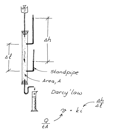
Note that we have added the hydraulic gradient into the mix, defined in the figure to the right.
This drawing shows a classic case of vertical, downward flow. The coefficient of permeability 

Upward Flow Example
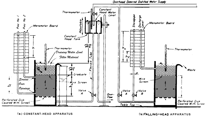
Consider the permeameter setup below. We will concentrate on the constant head permeameter on the left. The soil sample is in grey, with a length L and an area A.
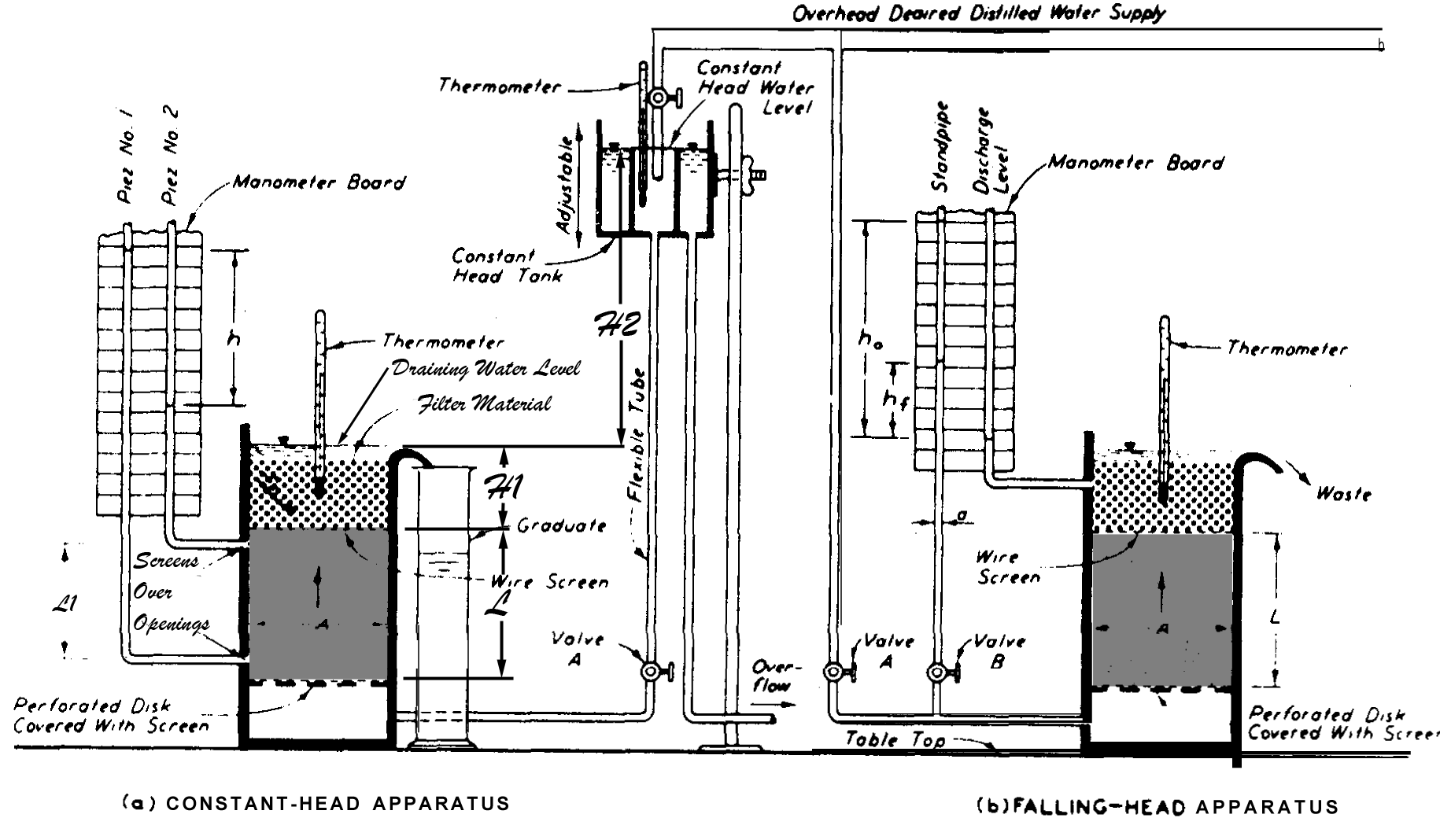
There is a distance H1 from the top of the soil sample to the surface of the water above it. There is an additional distance H2 from that water surface to the water surface of the constant head tank. We’ll do this three ways:
- Effective stresses using the “proper” way
- Effective stresses using the quick way
- Calculations of head at given points
The “Proper” Way (from Verruijt)
Now consider an example with the following parameters:
- H1 = 0.5 m
- H2 = 2.5 m
- L = 3 m

Compute the effective stress at a point halfway between the upper and lower surfaces of the soil sample.
First, we compute the total stress at the top of the soil, thus

Because the total stress at this point is due to free water, the pore water pressure 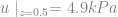

On the lower surface of the soil sample, the total stress is

The pore water pressure, however, is due to the free water that begins in the constant head tank and ends at the bottom surface of the soil, thus

The effective stress at this point is 61.9 – 58.8 = 3.1 kPa.
So how do we compute the effective stress at the midpoint in the soil sample? Let us revisit the equation
And determine the pore water pressure at the midpoint. We first want to compute the hydraulic gradient of the entire specimen, substituting yields

Solving for the hydraulic gradient yields 
Now we substitute this result back into the equation, changing the distance 

Adding the pore water pressure at the soil’s upper surface yields u = 4.9 + 26.95 = 31.85 kPa. The total stress at this point is

The effective stress is simply 33.4 – 31.85 = 1.55 kPa. Since this is the middle of the layer, we would expect this stress to be the average of the effective stress at the top of the soil and the bottom, which in fact is the case.
The Quick Way (which my students preferred)
We can show this by using a simpler method, by linearly interpolating between the properties of the top of the soil and the bottom. Since the point of interest is in the middle, we can use a simple average of the properties of the top and bottom. The averages are as follows:
- Total Stress:
- Pore Water Pressure:
- Effective Stress:


which are the same answers without some of the computational effort.
Computing the Hydraulic Head
Yet another way is to compute the hydraulic head at a given point. This is done as follows:
- At the top of the specimen, it’s simply the water depth from the surface = H1 = 0.5 m
- At the bottom of the specimen, it’s simply the distance from the surface of the constant head tank to the bottom of the specimen, thus = H1 + H2 + L = 0.5 + 2.5 + 3 = 6m
- The change in hydraulic head is the difference between the two, thus 6 – 0.5 = 5.5 m.
- Again since we’re in the middle of the specimen, the head at that point is the average of the two, thus Hcentre = (0.5+6)/2 = 3.25 m. If it were somewhere else in the specimen, use linear interpolation between the top surface and the bottom, it is a linear function of the distance between the two.
The pore water pressure is simply (3.25 m)(9.8 kN/m3) = 31.85 kPa, which is the same as before. The hydraulic gradient can be computed by rearranging Equation (3) and eliminating the unit weight of water to yield

Substituting yields 5.5/3 – 1 = 0.833, which is as before. Using hydraulic head eliminates the complications of the unit weight of water but hydraulic head may be an abstract concept for some students (but so in many cases is effective stress!) An example of hydraulic head “in action” can be seen in this experiment.
Comments
- The hydraulic gradient is very high; in fact, the critical hydraulic gradient for this soil is (per Soils in Construction Equation 9.4) 19/9.8 – 1 = 0.939, leaving us with a factor of safety of 1.13 (per Soils in Construction Equation 9.5.) This is reflected in the very low effective stresses that result. Had the critical hydraulic gradient been exceeded, the effective stresses would have been negative. Many “textbook” problems of this nature actually exceed any sensible range of hydraulic gradients because they don’t compute it as a part of the solution. The soil in this case is about to “boil” (or at least put significant upward pressure on the filter material.)
- Many students wonder why the formula for the hydraulic gradient
cannot be applied directly. The reason is simple: even with moving water, the direct hydrostatic effect due to gravity does not go away, and has to be considered. Thus we have the term
rather than just
.
- Had the flow been downward, the hydraulic gradient would have been negative, and the effective stresses would have increased relative to hydrostatic stresses rather than decreased.
- As long as the flow is vertical, this equation can be used with flow net type problems as well.
- The critical hydraulic gradient equation can be derived using this equation. As mentioned above, the critical hydraulic gradient is reached when the effective stresses in the soil are zero. Assuming that we’re starting at the upper surface where the effective stress is zero, at the lower surface of the soil sample (or soil element in a flow net) the effective stress is zero when the total stress and pore water pressure is zero, or

Solving for 

which is in fact the case.

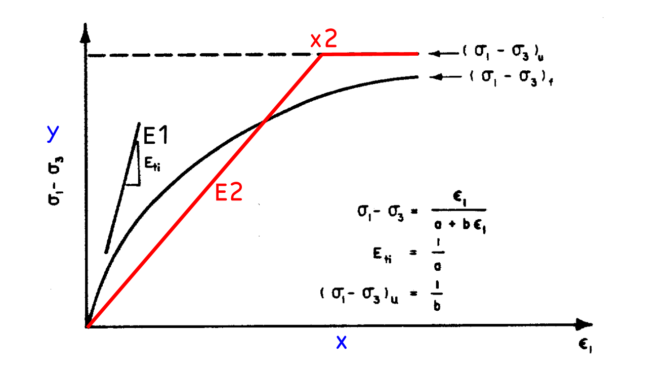


 line than to the x-axis. To do this we need first to rewrite the previous equation as
 from 0 to some value
  yields
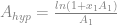
 ,
,

 , the ratio between the elastic modulus needed by elasto-plastic theory and the small-deflections modulus from the hyperbolic model. The bad news is that we need to know
  , which is the ratio of the small deflections modulus to the limiting stress. This implies that the limiting stress will be a factor in our ultimate result. Even worse is that


 and
and 
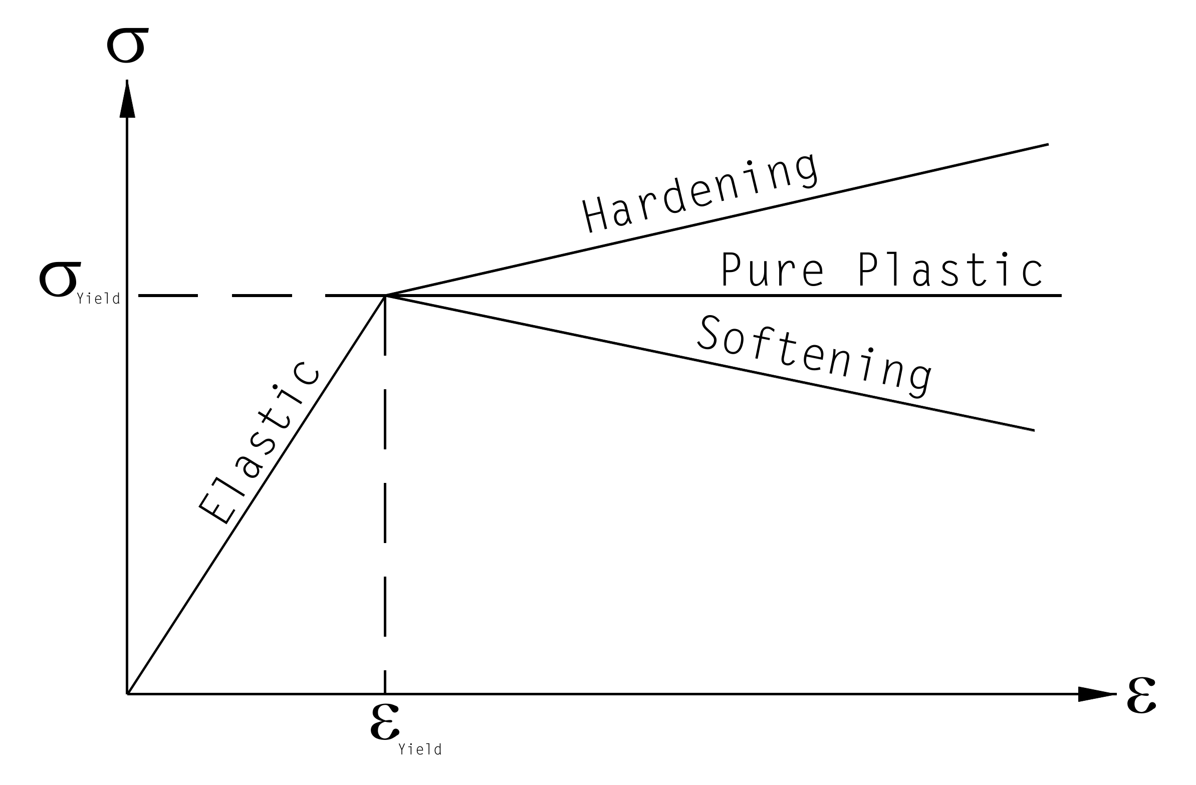
 . When
  , it is the case when the anticipated deflection is approximately equal to the “yield point.” For this case the ratio between the elasto-plastic modulus and the small-strain hyperbolic modulus is approximately 0.4. As one would expect, as
  likewise decreases. However, as the deflection increases this ratio’s increase is not as great.
 ) is 0.1″. Most “traditional” wave equation programs estimate the permanent set per blow to be the maximum movement of the pile toe less the quake. In the case of 120 BPF–a typical refusal–the set is 0.1″, which when added to the quake yields a total deflection of 0.2″ of a value of
  . This implies a value of
  . On the other hand, for 60 BPF, the permanent set is 0.2″, the total movement is 0.3″, and
  , which implies a value of
  . Cutting the blow count in half again to 30 BPF yields
  or
or  . Thus, during driving, not only does the plastic deformation increase, the effective stiffness of the toe likewise decreases as well.