I’m taking a break of my own from my review of the new NAVFAC DM 7.2 manual to present the video released by the ASCE Geo-Institute on the manual from its main coordinators and authors, Dan VandenBerge of Tennessee Tech University and Mike McGuire of Lafayette College.
Their comments will definitely be helpful in my reviews in the coming weeks.
One type of foundation that needs some explanation are floating or compensated foundations. Since they are sometimes referred to as “floating,” some fluid mechanics background is in order.
Fluid Mechanics
For ships to float, they obey Archimedes’ Law, where the weight of the ship is equal to the weight of water displaced by the hull of the ship. This is more thoroughly explained in my handout Buoyancy and Stability: An Introduction. I also go through all this in this video:
If the hull of the ship is rectangular, it’s also possible to compute the upward force of the water–which equals the downward force of the weight–by multiplying the hydrostatic pressure by the plan area of the ship, as is shown below. As the ship settles further and further into the water, the hydrostatic pressure increases until equilibrium is reached.
Illustrating Water Pressure Increasing in Proportion to the Draught
This last will be useful when we consider soils because, although box shaped ships are not so common, box shaped buildings and foundations are.
Turning to buildings, soils are an intermediate material between pure fluids and solids. Some are obviously more intermediate than others, but in softer soils they are more “fluid-like.” Let us consider the multi-storey building at the right.
If we consider that the soil acts as a fluid, then for the building to “float” in the soil the weight of the soil displaced must be greater than or equal to the weight of the building. The difference between ships and buildings is twofold. One, it is possible for a building to weigh less than the weight of the soil displaced and not get shoved upward until equilibrium is reached. The second is that, frequently, we use a “per unit area” approach to balance the equation and come up with the “draught” D of the building.
In this case we have a three-storey building where each storey has a unit weight of 10 kPa, or 10 kN per square metre of area. Multiplying the number of storeys n by the unit weight Δq yields 30 kPa. The soil weight is 18 kN/m3, or otherwise put the displaced soil exerts an “upward force” of 18 kPa/m of depth. Dividing the downward pressure by the unit weight yields a foundation depth/draught D = 1.67 m.
At this point it is worth noting that, depending upon the properties of the soil, it is not always necessary for the soil displaced to equal in weight to the building, but can be less. This is because soils, unlike fluids, have shear strength when not moving, an issue I discuss in my monograph Variations in Viscosity. An illustration of this is at the left.
Here we have a building with eight storeys and 10 kPa/floor, for a total pressure of 80 kPa. On the soil side we have a unit weight of 19 kN/m3 (after eliminating those pesky kilogram force units) and a foundation depth of 4 m, which results in an upward pressure of 76 kPa. The difference between the two is 4 kPa, not much but still enough to reduce the depth of the basement if the soil were a true fluid.
It’s first worth noting that an alternative way to look at the problem is that we are computing the total stress of the foundation at the base and then comparing it with the downward pressure of the building. That works for box like structures such as we are dealing with. If we have a more complex structure such as is shown at the right, we will have to adjust our strategy.
Beyond that, soils are routinely called upon to handle normal and shear stresses induced by the pressure exerted on the foundation. How well they do this is at the core of geotechnical foundation design. We must consider whether foundations will fail in bearing capacity, settlement or both. Bearing capacity is not as great of a problem with “large” structures such as mat foundations as it is with spread footings. Settlement, whether elastic or consolidation, is a major issue, and is something else that separates soils from fluids: rearrangement of the particles during volume change of the soil.
How much net pressure that is permissible is something that needs to be considered once it is established. Nevertheless, it is possible to use the soil’s own weight to help balance and support the structure during its useful life.
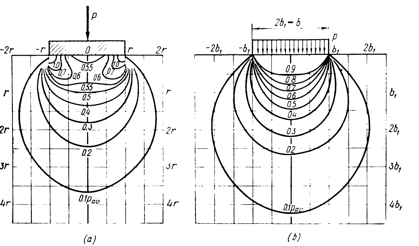
Figure 1. Isobars in Soil under Foundations a)absolutely rigid foundation, b)flexible foundation (from Tsytovich (1976))
View (a) shows a point load on a rigid foundation; it could be a distributed one too, as long as the load is concentric. In any case at the corners the vertical stress is infinite. In the real world one would expect the soil to go plastic long before that and the stresses to redistribute themselves, but we’ll stick with pure elasticity for the moment.
View (b) shows a distributed load on a flexible foundation. At the interface between the foundation and the soil the vertical stress is the load p, and it decreases the further you get away from the foundation. The strip load version of this is used to find the lower bound solution for bearing capacity in Lower and Upper Bound Solutions for Bearing Capacity.
This is the state of affairs for foundations which are either perfectly flexible or perfectly rigid. The truth is that neither one of these extreme approximations is really true. This is illustrated in the figure below.
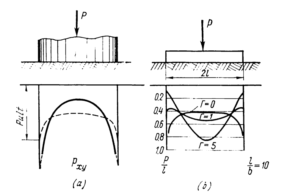
Figures 2. Diagrams of contact pressures a) under an absolutely rigid foundation, b) under foundations of various flexibilities. (From Tsytovich (1976))
View (a) shows the rigid foundation with the stresses at the base of the foundation as they would be in elastic theory (solid line) and those with some “real world” plasticity thrown in (dashed line.)
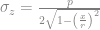
If the rigid foundation is circular, for a semi-infinite, elastic homogeneous space, the stress distribution is as follows:
(1)
where
vertical stress in soil
uniform pressure on foundation. With rigid foundations we can have a point load P and obtain the same result as long as the load is at the centroid of the foundation
distance from centroid
radius of foundation
The relationship between a distributed load and a point load at the centroid is
(2)
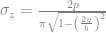
For a rigid strip foundation,
(3)
where
distance from centreline of strip load
width of foundations
If we define, as is done in Figure 1, the half width of the foundation as
(4)
then Equation (3) becomes
(5)
The line load can be computed as follows:
(6)
View (b) shows a foundation with varying flexibility and the effect that has on stress distribution at the base. The flexibility of the foundation is described by the variable . We’ll discuss how that’s calculated later but is a measure of the flexibility of the foundation.
is a totally inflexible (rigid) foundation
is a totally flexible foundation.
Before we get to that, let’s take a look at the other problem, that of a non-semi-infinite half space.
We now turn to the case of non-infinite spaces and rigid foundations. To deal with this problem we first present this table, from Tsytovich (1976):
Table 1. Contact Pressures under a Rigid Foundation on a Soil Layer of Limited Thickness (fractions of p, from Tsytovich (1976))
The simplest way to show how this is used is through an example. Consider the case of a rigid strip load 3m wide and having a uniform pressure p = 50 kPa. Determine the stress distribution under the soil if the layer under it (until is encounters a hard layer) is 3 m.
We start by considering Figure 1 and computing b1 = b/2 = 1.5m. We can thus say that h/b1 = 3/1.5 = 2. The ratio y/b1 varies from zero (at the centre of the foundation) to 0.95 (almost to the edge of the foundation, where the stress is infinite.) We compute the results for both the limited layer depth case (using Table 1) to the semi-infinite elastic space (using Equation 5) and tabulate the results below.
y/b1
y, m
Pressure Ratio (from chart)
Pressure, Limited Layer Depth, kPa
Pressure Ratio, Semi-Infinite Half-Space
Pressure, Semi-Infinite Half Space, kPa
0
0
0.705
35.25
0.637
31.831
0.1
0.15
0.707
35.35
0.640
31.991
0.2
0.3
0.714
35.7
0.650
32.487
0.3
0.45
0.725
36.25
0.667
33.368
0.4
0.6
0.744
37.2
0.695
34.730
0.5
0.75
0.773
38.65
0.735
36.755
0.6
0.9
0.818
40.9
0.796
39.789
0.7
1.05
0.891
44.55
0.891
44.572
0.8
1.2
1.029
51.45
1.061
53.052
0.9
1.35
1.366
68.3
1.461
73.025
0.95
1.425
1.869
93.45
2.039
101.941
Table 2. Results of Rigid Strip Load Example
The effect of the limited layer depth is primarily to flatten the pressure distribution across the base of the foundation. The pressures are greater for the limited layer depth case in the centre and less towards the edges. Inspection of Table 1 will show that this effect will become more pronounced as the layer below the foundation becomes thinner.
It is interesting to note that, while the right column is very close to Equation (5), it is not identical. The solution is shown in detail in Elastic Solutions Spreadsheet.
Foundation Flexibility
We have discussed the foundation flexibility coefficient . A general formulation of this is
(7)
where
Young’s Modulus and Poisson’s Ratio of the soil
Young’s Modulus and Poisson’s Ratio of the foundation
Half length of foundation
Width of foundation
moment of inertia of foundation
If we substitute
(8)
then
(9)
Making common substitutions of yields
(10)
which we will use in our subsequent calculations.
At this point it’s probably worth noting that relative flexibility between foundation and soil is most important in mat foundations. These days most of these will be designed using finite element analysis or some other numerical method, and rightly so. If the flexibility is more than rigid () the distribution of the load will come into play, and it is seldom that a foundation is uniformly loaded. In the case of eccentrically loaded foundations, even with rigid foundations the load is redistributed.
Nevertheless some kind of “back of the envelope” exercise is useful, not only for educational purposes but also for purposes of preliminary calculations. This is what we will do for stress distribution under a foundation with flexibility of . To begin we will present the following table, and as before we will illustrate its use with an example.
Table 2. Relative Pressures for Half-Span l of Flexible Uniformly Loaded Beams on a Soil Layer of Limited Thickness H, with a Distribution Diagram (from Tsytovich (1976))
Let’s first dispense with the columns labelled . These are purely flexible foundations, the pressure on the soil is the same as the pressure on the foundation. The rest of these are for foundations with varying degrees of rigidity, from purely rigid foundations () to those where, as increases, the flexibility of the foundation does also.
Since we are dealing with rectangular foundations, with a uniform pressure p the stress distribution is symmetrical about the centroidal axes of the foundation. The ratio is the fraction of the distance between the centroidal axis and the long end of the foundation, and in this case is divided into eight equal segments.
Figure 3. Example of Shape and Rigidity Factors I for Calculating Settlements of Points on Loaded Area at the Surface of an Elastic Half-Space (from NAVFAC DM 7.01)
The parameters necessary are as follows:
The Young’s Modulus for concrete is approximately 720,000 ksf.
We will assume that the foundation is 0.45′ (5.4″) thick for reasons that will become apparent.
The half length of the foundation is 10′, which means that, for Table 2, .
We will use the approximate value of in Equation 10. Substituting, , which avoids a great deal of interpolation.
Using Table 2 and making the appropriate substitutions yields the following results.
Fraction of Pressure
Soil Vertical Reaction, ksf
Rigid Foundation
Flexible Foundation
Rigid Foundation
Flexible Foundation
0.0625
0.828
0.876
1
3.312
3.504
4
0.1875
0.829
0.874
1
3.316
3.496
4
0.3125
0.836
0.874
1
3.344
3.496
4
0.4375
0.837
0.866
1
3.348
3.464
4
0.5625
0.857
0.87
1
3.428
3.48
4
0.6875
0.899
0.893
1
3.596
3.572
4
0.8125
0.987
0.958
1
3.948
3.832
4
0.9375
1.927
1.791
1
7.708
7.164
4
Table 3 Results of flexibility study
From this result we note the following:
As a practical matter, the results of the rigid foundation and that for are not that different, but they are different from the flexible foundation (.)
The foundation is fairly thin to be considered “rigid.” One possibility is that the Young’s Modulus for the soil is very low. If we were to increase this by a factor of 10 to 200 ksf, we would achieve the same value for with a foundation 1′ thick, which is still rigid relative to the soil.
By the time the foundation is approaching being purely flexible.
Although it would be nice to be able to determine the soil stress distribution under a foundation, for preliminary purposes it is probably not necessary since other methods of analysis must be done. Nevertheless the rigidity coefficient is potentially useful as a starting point to determine whether a foundation can be considered rigid or flexible.
Table 3. Relative Mat Stiffness and Behavior (after Brown (1969,) Frazer and Wardle (1976))
A different notation for the stiffness factor is noted, but the similarity between the equations (especially that of the rectangular foundation) and Equation 10 is unmistakable. This is because there are common sources to both. For rectangular foundations the relationship between the two can be found by the equation
(11a)
or conversely
(11b)
Thus, considering rectangular foundations in Table 3, a foundation is flexible if , rigid if , and intermediate between these values. For practical purposes, an intermediate foundation has , it is rigid below this and flexible above.
One interesting difference is that Table 3 uses the short dimension B while Equation 10 uses the long half dimension l. For the square foundation in the example this isn’t a problem. However, it makes sense that the longer dimension drives the flexibility–and the bending moments–of the foundation.
In any case the behavior of the foundation can be affected by the relative rigidity of the mat and the soil under it. As NAVFAC DM 7.1 notes:
As indicated in Table 5-8, mats with low stiffness ratios can be considered completely flexible. Flexible mats will apply a relatively uniform pressure distribution, and the center, edges, and corners will settle differentially. Mats with high values of * will act in a rigid manner and will tend to settle uniformly.
* Or low values of
Two other factors need to be considered: the bending stresses in the mat (which is also affected by the reinforcement scheme) and the maximum stresses in the soil. The bending stresses in the mat needs to be considered on a case-by-case basis. Conventional wisdom may indicate that rigid mats would have larger bending stresses, but flexible mats are probably relatively thin and bending stresses may increase in these cases. The maximum stress in the soil immediately around the mat are higher with rigid mats than with flexible ones, especially along the edges. However the soil stresses that most influence the behaviour of the mat may be those which induce the largest settlements, such as those in, say, soft clay layers.
It’s happened again: the paper “Vibratory and Impact-Vibration Pile Driving Equipment” has been cited by Mohammed Al-Amrani and M Ikhsan Setiawan in their paper “Prefabricated and Prestressed Bio-Concrete Piles: Case Study in North Jakarta.” The abstract of their paper is here: In this research, we will talk about Prefabricated and Prestressed Concrete piles in general and […]
It comes around every year, but this time it’s very special: today is the twenty-fifth anniversary of the start of this site. I wrote pieces of this for the tenth anniversary and the twentieth anniversary and one in the wake of COVID, which did as much as anything to move it in a more educational direction and not just a document download site.
You’d think that a site this old would have run its course, but it hasn’t: it continues to grow in traffic and popularity. The shift to a more educational emphasis has paid off, especially in traffic from outside of the U.S.. This is the fulfillment of a dream.
Want to support the site? Buy the books listed in the sidebar (or at the bottom, for those of you on mobile devices.) That’s all we ask. Again, as with my class videos, thanks for visiting and God bless.


 (1)
(1) vertical stress in soil
 uniform pressure on foundation. With rigid foundations we can have a point load P and obtain the same result as long as the load is at the centroid of the foundation
 distance from centroid
 radius of foundation
 (2)
(2) (3)
(3) distance from centreline of strip load
 width of foundations
 (4)
(4) (5)
(5) (6)
(6) . We’ll discuss how that’s calculated later but
  is a totally inflexible (rigid) foundation
 is a totally flexible foundation.
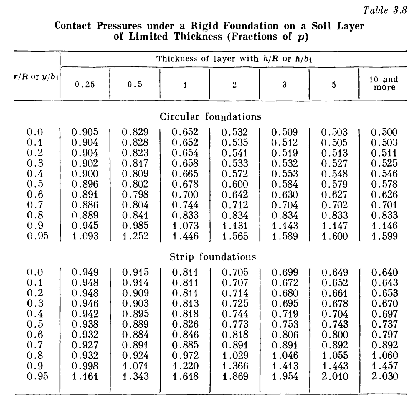
 (7)
(7) Young’s Modulus and Poisson’s Ratio of the soil
 Young’s Modulus and Poisson’s Ratio of the foundation
 Half length of foundation
 moment of inertia of foundation
 (8)
(8) (9)
(9) yields
 (10)
(10) ) the distribution of the load will come into play, and it is seldom that a foundation is uniformly loaded. In the case of eccentrically loaded foundations, even with rigid foundations the load is redistributed.
 . To begin we will present the following table, and as before we will illustrate its use with an example.
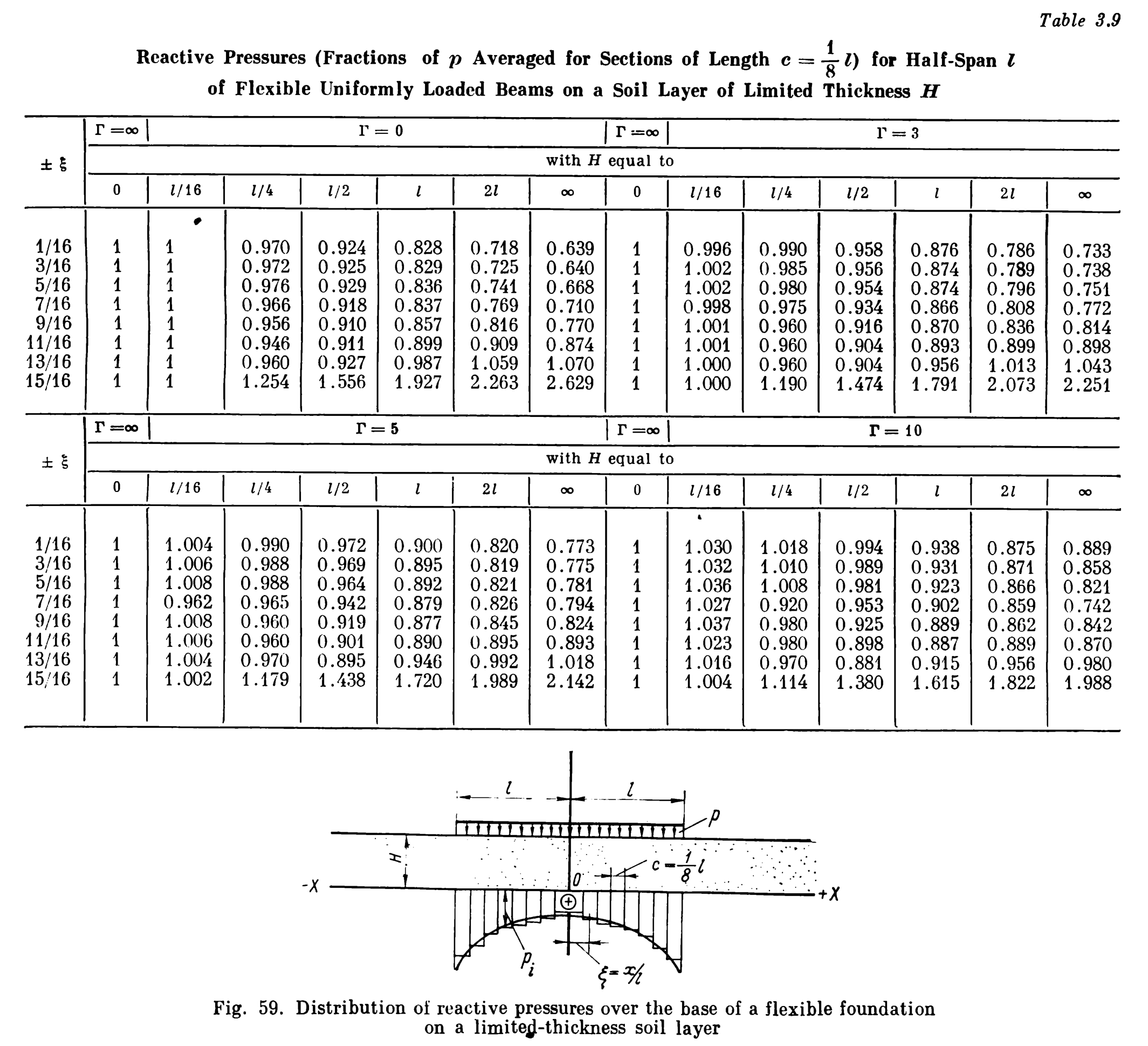
 is the fraction of the distance between the centroidal axis and the long end of the foundation, and in this case is divided into eight equal segments.
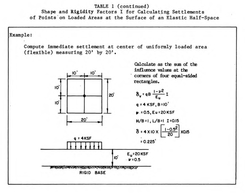
 of the foundation is 10′, which means that, for Table 2,
  .
. , which avoids a great deal of interpolation.

 the foundation is approaching being purely flexible.
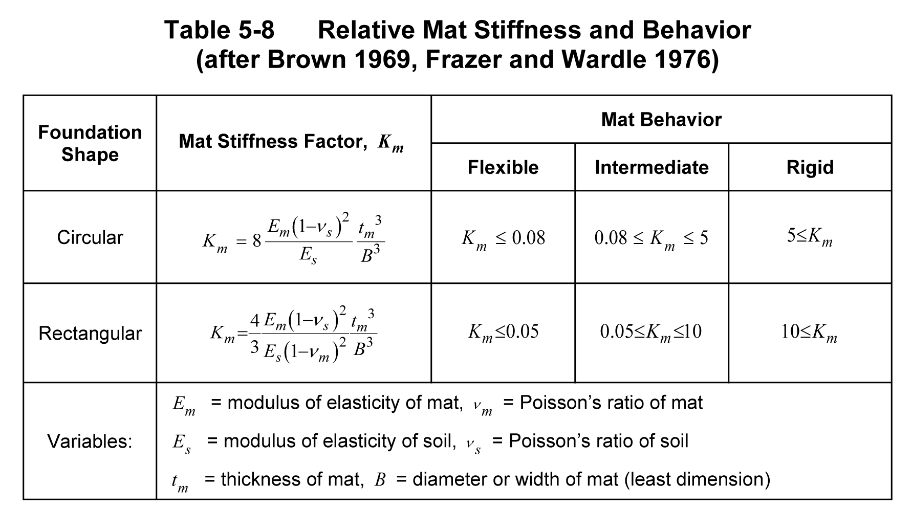
 (11a)
(11a) (11b)
(11b) , rigid if
  , and intermediate between these values. For practical purposes, an intermediate foundation has
  , it is rigid below this and flexible above.
 * will act in a rigid manner and will tend to settle uniformly.
