One of the reasons I was interested in teaching Statics at Lee University was because I was continually disappointed at my students’ memory of their statics. Statics is crucial in the design and analysis of geotechnical structures, and most of the problems–at the undergraduate level at least–aren’t that involved, or at least I thought they weren’t. A great deal of the problem is that geotechnical statics usually involves converting distributed loads into resultants, which Statics–and Mechanics of Materials for that matter–generally associate this with beam problems, not always the case with geotechnical problems.
Another culprit is that Statics, in the U.S. at least, is a vector proposition from the start. At the University of Tennessee at Chattanooga where I taught, it was called “Vector Statics,” which gives the game away early. (At Lee we use the same book and teach the same material, but simply title it “Statics.”)
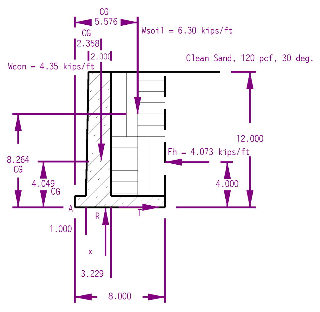
But what if we applied a vector approach to a simple geotechnical problem? That’s what we’re going to do here with a concrete gravity wall. I will use the method outlined in my post A Simplified Method to Design Cantilever Gravity Walls. You can refer to the theory there, I will try to keep it to a minimum. The wall is pictured at the top of the post, I will reproduce it below.
Analysing Overturning
We have three forces acting on the wall:
- The weight of the gravity wall itself, Wconc
- The weight of the soil trapped by the heel of the wall, Wsoil
- The lateral force of the soil on the wall, Fh
Forces 1 and 2 are determined by computing the cross-sectional area of the concrete and soil and multiplying each by the unit weight as shown above, and then converting the result to a vector force and placing it at the centroid of the area (another Statics topic.) Instead of the “manual” approach in A Simplified Method to Design Cantilever Gravity Walls, the was was drawn in CAD and both the areas and centroids were determined automatically. You can see the magnitudes and locations of those resultants above.
The lateral force of the soil is computed using Rankine’s theory. The first thing is to determine the working internal friction angle of the soil by applying the Shear Mobilisation Factor SMF. Assuming an SMF of 2/3, that friction angle changes from the 30 degree one shown above to a 21.05 degree one, which is applied to the formula for Rankine active pressures for level backfill,

Doing that results in a kh = .471. The force on the wall is then determined by the formula

The division by two reflects the fact that soil effective stress (and thus lateral earth pressure) increases linearly with depth (like a fluid,) creating a triangular distribution (yet another concept from Statics.)
At this point there the resisting forces R and T are not defined. The forces themselves are easily computed by summing forces in the x and y directions. Doing this, we have


The location of F–along the surface of the footing–is evident. The location of R is not; it is some distance x from the toe (Point “A”) of the footing. We can obtain x by summing moments around Point “A,” and with a vector method that means taking cross products of the moment arms with the forces.
Converting both the moment arms r and the forces to vector notation yields the following:
- Concrete Weight: r = 2.358 i + 4.049 j, Wcon = −4.35 j
- Soil Weight: r = 5.576 i + 8.264 j, Wsoil = −6.30 j
- Lateral Earth Pressure: r = 8 i + 4 j, Fh = −4.073261616 i
- Vertical Footing Force: r = x i, R = 10.65 j (Equation (3a))
The force T does not enter into this because its line of action runs through Point “A,” thus its moment is zero as its moment arm is zero.
The cross product moments around the toe (Point “A” in the drawing) are as follows:
- Concrete Weight:
- Soil Weight:
- Lateral Earth Pressure:
- Vertical Footing Force:
![\left [\begin {array}{ccc} i&j&k\\{\medskip} 2.358& 4.049&0 \\{\medskip}0&- 4.35&0\end {array}\right ] = -10.257 k](https://s0.wp.com/latex.php?latex=%5Cleft+%5B%5Cbegin+%7Barray%7D%7Bccc%7D+i%26j%26k%5C%5C%7B%5Cmedskip%7D+2.358%26+4.049%260+%5C%5C%7B%5Cmedskip%7D0%26-+4.35%260%5Cend+%7Barray%7D%5Cright+%5D++%3D+-10.257+k+&bg=ffffff&fg=777777&s=0&c=20201002)
![\left [\begin {array}{ccc} i&j&k\\{\medskip} 5.576& 8.264&0\\{\medskip}0&- 6.3&0\end {array}\right ] = -35.129k](https://s0.wp.com/latex.php?latex=%5Cleft+%5B%5Cbegin+%7Barray%7D%7Bccc%7D+i%26j%26k%5C%5C%7B%5Cmedskip%7D+5.576%26+8.264%260%5C%5C%7B%5Cmedskip%7D0%26-+6.3%260%5Cend+%7Barray%7D%5Cright+%5D+%3D+-35.129k+&bg=ffffff&fg=777777&s=0&c=20201002)
![\left [\begin {array}{ccc} i&j&k\\{\medskip}8&4&0\\{\medskip}- 4.073&0&0\end {array}\right ] = 16.293k](https://s0.wp.com/latex.php?latex=%5Cleft+%5B%5Cbegin+%7Barray%7D%7Bccc%7D+i%26j%26k%5C%5C%7B%5Cmedskip%7D8%264%260%5C%5C%7B%5Cmedskip%7D-+4.073%260%260%5Cend+%7Barray%7D%5Cright+%5D+%3D+16.293k&bg=ffffff&fg=777777&s=0&c=20201002)
![\left [\begin {array}{ccc} i&j&k\\{\medskip}x&0&0\\{\medskip}0& 10.65&0\end {array}\right ] = 10.65 x k](https://s0.wp.com/latex.php?latex=%5Cleft+%5B%5Cbegin+%7Barray%7D%7Bccc%7D+i%26j%26k%5C%5C%7B%5Cmedskip%7Dx%260%260%5C%5C%7B%5Cmedskip%7D0%26+10.65%260%5Cend+%7Barray%7D%5Cright+%5D+%3D+10.65+x+k+&bg=ffffff&fg=777777&s=0&c=20201002)
Summing these moments,

Solving yields x = 2.732′. At this point we need to determine whether this is an acceptable location or not for the force. The goal is for the pressure to be positive (downward) along the entire surface of the footing. There are two ways of determining this:
- Computing the pressures on each end of the footing, as is done in A Simplified Method to Design Cantilever Gravity Walls.
- Determining whether the force is in the “middle third” of the foundation, as is discussed in the Soils and Foundations Reference Manual.
We will do the latter. The middle third of this foundation falls between 2.67′ < x < 5.33′, so the vertical footing force is within the middle third (barely.) As I noted in A Simplified Method to Design Cantilever Gravity Walls, “In this case we make a common assumption that, as long as the resultant force of the wall is within the kern and there are no negative pressures on the base, overturning will not be experienced. It is certainly possible to do an explicit overturning analysis to check this result.”
Analysing Sliding
With the lack of keys or deep foundations, the only lateral resistance to sliding is the friction force T. We computed that force based on Equation (3b,) but in reality that force cannot exceed–and there should be a factor of safety in that inequality–the frictional force possible, which is defined by the equation

in which case

Equation (5) is written in “mechanical engineers format.” Geotechnical engineers understand all too well the concept of a friction angle. In my post Explaining the Relationship Between the Coefficient and the Angle of Friction I relate the two from a non-geotech standpoint; we can turn Equation (5) into a more “geotech-friendly” form by noting that

Let us assume that the value of 


Observations
- The use of vectors for this problem is overkill from a computational standpoint. It also requires locating the centroid/CG of the two regions in both the x- and y-directions, although with using CAD this is trivial. On the other hand doing it using vectors is more “bullet proof” in that the student is not required to “think” but just “plug and chug” without having to identify lines of action and perpendicular moment arms.
- The fact that the word “barely” appears in both analyses should inspire some additional conservatism in the design. The simplest way to improve the situation would be to move the heel to the right, which would shift the resisting forces away from the toe (and thus increase their resisting moment) and also put the footing force resultant deeper into the middle third.
- Both bearing capacity and settlement of the wall’s foundation, the methodology for which are discussed in A Simplified Method to Design Cantilever Gravity Walls, are beyond the scope of this post. Also beyond the scope of this post is the structural design of the wall and of course the global stability of the wall as well.


 at a distance
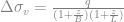
  below the centre of the foundation, the equation for a rectangular foundation of width B and length L (can be interchanged, but conventionally B is the smaller of the two) for a load Q on the surface is given by the equation
 (1)
(1) (2)
(2) but the solution is the same.
 the equation reduces to
 (2a, Continuous Foundations)
 . By substitution into Equation (1),
  . If we compute the unit load to be
 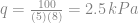 , substitution into Equation (2) yields the same result.
 and all other variables the same is
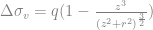 (3)
(3)