In an earlier post we discussed consolidation settlement. For situations where soil a) decreases its volume due to rearrangement of the particles and b) does so over a relatively long period of time due to difficulties in expelling pore water pressures, we need to know how long it takes to reach maximum settlement, in addition to know what that settlement is and what deflections we might achieve along the way.
This is generally a two part process: a) determining the dissipation of pore water pressure and b) determining the amount of settlement at a given time. This post will focus on the first part of the process; we will deal with the second in a later post. This is a well-worn path in geotechnical engineering but hopefully this derivation is a little simpler than others.
Developing the Differential Equation
Relating Porosity to Strain
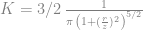
Let us begin by considering the system above (from Tsytovich (1976)), a uniformly loaded soil layer which is saturated (always) and clay (usually.) The first thing we need to note is that, while the diagram uses z as the variable of length in the vertical direction, from this post we will use the variable x (sorry for the confusion.) The second thing is that we assume the water and the solids to be incompressible. The third thing is that all the changes that take place do so because of changes in the voids where the water is resident. We first note the definition of porosity as

where
- n = porosity
- Vv = volume of voids
- Vt = total volume
That being the case, the relationship between the porosity of the soil (due to changes in the volume of the voids) and the flow rate of the water can be expressed as

We can envision a differential volume having a height x and an area A. Since the problem is one-dimensional, the areas cancel out and the ratio of the void height to the total height is

where
- xv = height of the voids
- xt = height of the solids
We want to determine the change in porosity from some state 0 to some state 1, just as we did with void ratio in this post. That change can be expressed as follows:

We can assume that the change in void volume xv0 – xv1 << xt0, in which case Equation (4) can be simplified to

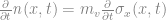
Now we can say, for the small increments we are dealing with here, that the change in strain is equal to the change in porosity,

From this and our previous post, we can thus use the change in strain to come to the following:

Stating this differentially,
In this way we emphasise that both porosity and uniaxial stress are functions of depth and time. We now combine Equations (2) and (8) to yield

Including Permeability
Darcy’s Law (or more properly d’Arcy’s Law) states that
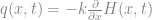
where k is the coefficient of permeability and H is the hydraulic head. We then combine Equations (9) and (10) to obtain

Noting that

where 

Putting It All Together
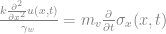
We now define the parameter

At this point we need to stop and make an observation: this whole process wouldn’t be worth too much if 


Tidying up the Physics, Governing Equation, Boundary and Initial Conditions, and the Solution
It should be evident that getting to Equation (15) was a major triumph for geotechnical theory. But it’s also evident that there’s one glaring problem: the dependent variable on the left hand side is not the same as the one on the right. It is here that we need to clarify some assumptions behind our equations.
A basic assumption in consolidation theory is that, when the load at the surface is applied, all of this additional load is initially borne by the pore water pressure. Because of the aforementioned permeability, the water will want to “head for the exits,” i.e., the permeable boundaries of the layer being compressed. When the particles have rearranged themselves and the excess pore water has been squeezed out, the settlement should stop (until secondary compression kicks in.) During this process the load on the pore water is being progressively transferred to the soil particles until consolidation has stopped (which, in theory, it never does, as we will see) and the load is completely handed off to the particles.
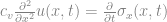
That being the case, the consolidation equation (15) should be rewritten as
At this point we should invoke the effective stress equation
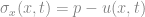
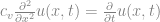
where p is the applied pressure, and do the following to determine the time and distance history of the vertical stress 
- Determine the solution of Equation (16), which will be our governing equation.
- Determine the initial and boundary conditions for the problem.
- Solve the problem for
There are several ways to solve the governing equation for this problem. Verruijt employed Laplace Transforms to accomplish this; these are very useful, as was demonstrated by Warrington (1997) for the wave equation. For this analysis, we will use separation of variables, a method which is not as fundamental as one might like (this is a demonstration of a method that is) but which is easier to follow than most of the others.
The separation of variables begins by assuming the solution is as follows:

This means that the solution is a product of two functions, one of time and the other of distance, and that those functions are separate one from another. Substituting this into Equation (16) and rearranging a bit yields

Since the left and right hand sides are equal to each other, they are equal to a third variable, which we will designate as 


The solutions to these equations are, respectively,


We need to pause and consider the boundary conditions. As the problem is shown at the top of the article, the boundary conditions are as follows:


Equation (22a) represents a Dirichelet boundary condition and Equation (22b) represents a Neumann boundary condition. While the equation for 
- Mirror the problem shown above at x = h so that you have two permeable boundaries.
- You now have a layer of 2h thickness with Dirichelet boundary conditions on both sides. At the centre of this new layer, there is no flow; the water above it flows upward, and the water below flows downward.
- Problems in the field can have either one or two permeable boundaries. The distance h is NOT the thickness of the layer but the longest distance the trapped pore water must travel to escape. Confusing h with the thickness of the layer is a common mistake and should be avoided at all costs.
That said, the second boundary condition is now

Returning to Equation (21a), because of Equation (22a) 


This is the square root of the eigenvalues. Any integer value of n > 0 is valid for this, and we will have recourse to them all to produce a complete orthogonal set (Fourier Series) to solve the problem.
This change will affect both Equations (21a) and (21b). Combining constants into the coefficient 
At this point we need to consider our initial conditions 

Substituting 

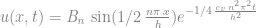
Substituting this into Equation (24) and taking the complete sum, we have at last

More simply we can say that

The vertical pressure on the soil skeleton is determined by combining Equations (17) and (28) to yield

It is interesting to note that, although Equation (27) includes all positive non-zero values of n, only the odd ones end up in Equations (28) and (29). For even values of n, 
Conclusion
At this point we have derived the equations of pressure dissapation for consolidation settlement. In a future post we will deal with the second part of the problem, namely how much of the total anticipated settlement has taken place at any given time from initial loading.
Reference
Kreyszig, E. (1988) Advanced Engineering Mathematics. Sixth Edition. New York: John Wiley and Sons
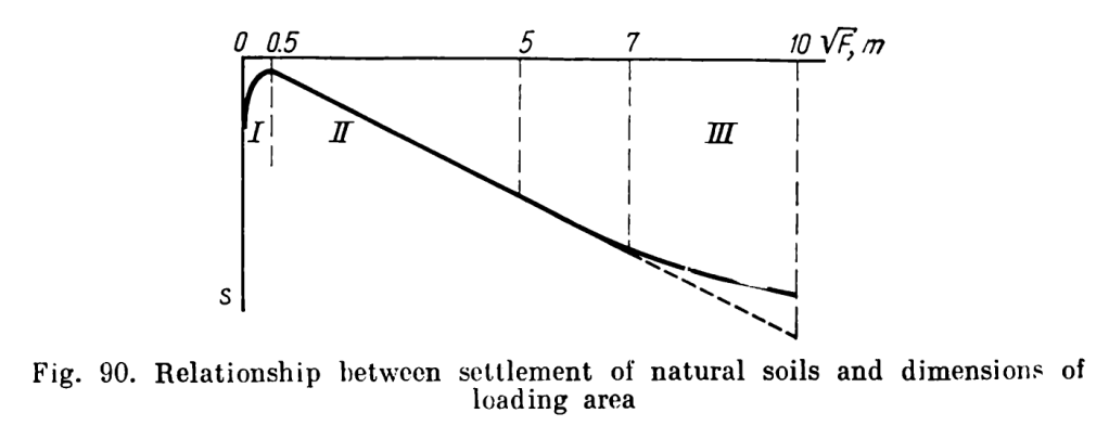
 and at average pressures on soil correspond to the compaction phase, i.e., are very close to the theoretical ones; and III — the region of areas larger than 25-50 m2, where settlements are smaller than the theoretical ones, which may be explained by an increase of the soil modulus of elasticity (or a decrease of deform ability) with an increase of depth. For very loose and very dense soils these limits will naturally be somewhat different.
 (1)
(1) settlement of the foundation at the point of interest
 influence factor, given in the table below
 uniform pressure on the foundation
 smaller dimension of rectangle or dimension of square side
 Poisson’s Ratio of the soil
 Modulus of elasticity of the soil
 are shown below.
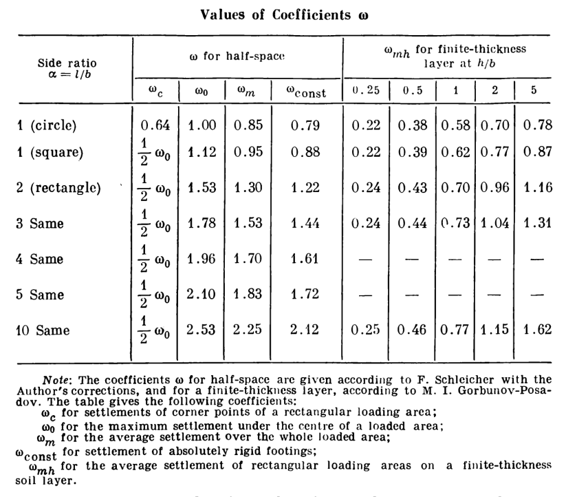
 (2)
(2) is the spring constant of the soil and
  is the foundation’s radius. If we break it down further, as is done in
  (3)
(3)