Lateral Earth Pressure Coefficients for Beta Methods in Sands

In our last post we considered some basic concepts behind beta methods for determining beta coefficients for estimating shaft friction for piles in sands. The idea is that the unit friction along the surface of the pile can be determined at any point by the relationship

$f_s = \beta \sigma'_{vo}$

where $f_s$ is the unit shaft friction, $\sigma'_{vo}$ is the vertical effective stress, and $\beta$ is the ratio of the two, which can be further broken down as follows:

$\beta = K tan \phi$

where $K$ is the lateral earth pressure coefficient and $\phi$ is the internal friction angle of the soil. Our last post showed that, when compared with empirically determined values of $\beta$ , values of $K$ determined from more conventional retaining wall considerations are not adequate to describe the interaction between the shaft of the pile and the soil.

Needless to say, there has been a good deal of research to refine our understanding of this relationship. Also, needless to say, there is more than one way to express this relationship. The formulation we will use here is that of Randolph, Dolwin and Beck (1994) and Randolph (2003), and was recently featured in Han, Salgado, Prezzi and Zaheer (2016). The basic form of the lateral earth pressure equation is as follows:

$K = K_{min} + (K_{max} - K_{min}) e^{-\mu \frac {L-z}{d}}$

Let’s start on the right end of the equation; the exponential term is a way of representing the fact that the maximum shaft friction (with effective stress taken into account) is just above the pile toe and decays above that point to the surface of the soil. This was first proposed by Edward Heerema (whose company was instrumental in the development of large steam and hydraulic impact hammers) in the early 1980’s. (For another paper of his relating to the topic, click here.)

In any case the variables in the exponential term are as follows:

$\mu =$ rate of exponential decay, typically 0.05
$L =$ embedded length of pile into the soil
$z =$ distance from soil surface to a given point along the pile shaft. At the pile toe, $L = z$ and $L-z = 0$ , and the exponential term becomes unity.
$d =$ “diameter” of the pile, more commonly designated as B in American textbooks.

$K_{min}$ is the minimum lateral earth pressure coefficient. It, according to Randolph, Dolwin and Beck (1994) “can be linked to the active earth pressure coefficient.” Randolph (2003) states that its value lies in the range 0.2-0.4. We stated in our previous post that

$K_a = \frac {1 - sin \phi} {1 + sin \phi}$

How do these two relate? Although in the last post we produced extensive parametric studies on these, a simpler representation is to compare the active earth pressure coefficient with Jaky’s at-rest coefficient, which is done below.

Beta Image 4

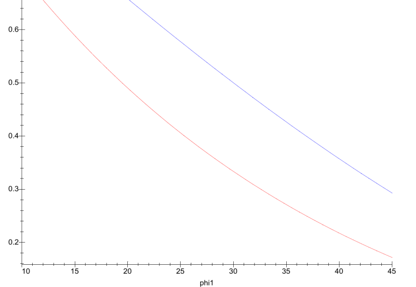
The at-rest coefficient from Jaky is in blue and the active coefficient from Rankine is in red. The range of $0.2 < K_a < 0.4$ approximately translates into $25^\circ < \phi < 45^\circ$ , which is a wide range for granular soils but reasonable.

That leaves us $K_{max}$ . Randolph, Dolwin and Beck (1994) state that

$K_{max} = S_t N_q$

$N_q$ , of course, is the bearing capacity factor at the toe. It may seem odd to include a toe bearing capacity factor in a shaft equation, but keep in mind that cavity expansion during pile installation begins (literally) with an advancing toe. Typically $8 < N_q < 40$ depending upon whether the sand is loose (low end) or dense (high end.) $S_t$ “is the ratio of the radial effective stress acting in the vicinity of the pile tip at shaft failure to the end-bearing capacity.” Values for $S_t$ vary somewhat but generally centre around 0.02. This in turn implies that $0.16 < K_{max} < 0.8$ . Inspection of the complete equation for $K$ shows that, if $L = z$ and the exponential term is at its maximum, $K_{min}$ cancels out and the range of $K_{max}$ is a range for $K$ .

Comparing this result to the graph above, for larger values of $\phi$ these values of $K$ are greater than those given by Jaky’s Equation, which is what we were looking for to start with. To compute $\beta$ , we obviously will need to multiply this by $tan \phi$ (or $tan \delta$ ). For, say, $\delta = 35^\circ$ , this leads to $\beta_{max} = 0.8 \times tan 35^\circ = 0.56$ . By way of comparison, using Jaky’s Equation for $K, \beta = (1 - sin 35^\circ) tan 35^\circ = 0.30$ .

From this we have “broken out” of Burland’s (1973) limitation on $\beta$ , which was useful for him (and will be useful to us) for some soils but creates problems with higher values of $\phi$ Although some empirical methods indicate higher values for $\beta$ , if we consider variations in $S_t$ and other factors, this differential can be minimised, and in any case this is not a rigourous excercise but a qualitative one.

One thing we should further note–and this is important as we move forward–is that there is more than one way to compute $K_{max}$ . Randolph (2003) states that, when CPT data is available, it can be computed as follows for open-ended piles:

$K_{max} = 0.01 \frac {q_c}{\sigma'_{vo}}$

where $q_c$ is the cone tip resistance. Randolph (2003) recommends the coefficient be increased to 0.015 for closed-ended piles. Making generalisations from this formulation is more difficult than the other, but the possibility of using this in conjunction with field data is attractive indeed.

At this point we have a reasonable method of computing $\beta$ coefficients. However, we still have the issue of clay soils to deal with, and this will be done in a subsequent post.

References

In addition to those previously given, we add the following:

Han, F., Prezzi, M., Salgado, R. and Zaheer, M., (2016), “Axial Resistance of Closed-Ended Steel-Pipe Piles Driven in Multilayered Soil“, Journal of Geotechnical and Geoenvironmental Engineering, DOI: 10.1061/(ASCE)GT.1943-5606.0001589.
Randolph, M., Dolwin, J., Beck, R. 1994, ‘Design of driven piles in sand’, GEOTECHNIQUE, 44, 3, pp. 427-448.
Randolph, M. 2003, ‘Science and empiricism in pile foundation design’, GEOTECHNIQUE, 53, 10, pp. 847-875.