When you’ve taught any course for as long as I taught Soil Mechanics and Foundation Design and Analysis, you’ll sometimes get inquiries from your students about topics that you either didn’t cover or they might have missed. (Many comforted themselves during the course with the thought that “I’ll never go into geotech,” only to have it be their first job.) This topic came from a student from Florida (which is, of course of special interest for a long list of reasons, esp. since I grew up there) who saw on a geotech report about bearing pressure on a shallow foundation (in this case, a pool) citing the net bearing pressure on the foundation.
Using the notation above, the pressure p is the gross bearing pressure on the foundation. The pressure p0 is the effective stress at the base of the foundation. The difference between the two is Δp, which is the net bearing pressure on the foundation.
So how is this relevant to foundation design? In the case of Schmertmann’s Method, it is a part of the method. For bearing capacity, the Soils and Foundations Reference Manual has the following to say:
The net ultimate bearing pressure is the difference between the gross ultimate bearing pressure and the pressure that existed due to the ground surcharge at the bearing depth before the footing was constructed, q (= γaDf). The net ultimate bearing pressure can thus be computed by subtracting the ground surcharge (q) from Equation 8-6:
The structural designer will typically include the self-weight of the concrete footing and the backfill over the footing (approximately equal to γaDf) in the loads that contribute to the applied bearing stress. Therefore, if the geotechnical engineer computes and reports a net ultimate bearing pressure, the effect of the surcharge directly over the footing area is counted twice. Reporting an allowable bearing capacity computed from a net ultimate bearing pressure is conservative and generally not recommended provided that a suitable factor of safety is maintained against bearing capacity failure. If the geotechnical engineer chooses to report an allowable bearing capacity computed from a net ultimate bearing pressure, this fact should be clearly stated in the foundation report.
In general, the ultimate capacity is the more conservative option to use. Combined with the difficulties associated with bearing capacity analysis, I decided not to emphasise net bearing capacity in my teaching. Additionally, for a small pool like the one we had in Palm Beach, bearing capacity failure is remotely possible. For a large (say, Olympic) size pool, we’re dealing with something approaching a mat foundation, and these generally fail in settlement, as noted in Foundation Design and Analysis: Shallow Foundations, Other Topics.
This post has been a long time coming. I’ve been teaching engineering for a quarter century now, and when not doing that developing sites like this so that engineers (and others) can learn more about design and construction of geotechnical structures (and all structures, to varying degrees, are geotechnical unless they float on the water, in the air or in space.)
I come from a long time of technically educated people, as visiting my sites vulcanhammer.info and Chet Aero Marine will show. My great-grandfather learned the basics from Smith’s Mechanic at the University of Illinois in the 1870’s and both he and his brother had successful careers as naval architects. So I come to this debate with a long family history in this profession and many years of experience in the design and application of construction equipment, which is why my teaching straddles both Civil and Mechanical engineering. Many of those who have visited this site are familiar with my Soil Mechanics, Soil Mechanics Laboratory and Foundations courses. After teaching these for a long time, it was evident that our students weren’t “getting it” on what I thought were fundamental concepts. Moving to Lee University and teaching Statics and Dynamics only confirmed those suspicions. Added to my experience with Fluid Mechanics Laboratory and later Fluid Mechanics and this post is the sum of my reflections on this experience.
The growth in the use of numerical methods while the curriculum still emphasizes the use of “hand calculations.” A lot of that is driven by testing; as my CFD professor said after a disastrous midterm (and it was a 500 level course!) testing isn’t perfect but it’s the best thing we have to evaluate whether students are learning the material. Conversely, the problem with simply relying on numerical methods without any recourse at all is that engineers tend to regard results that a computer produces come from Mt. Sinai (the “black box” phenomenon”) and this does not lead to good engineering practice.
We all too frequently lose sight of the fact that our first purpose is to teach people how to think, not just how to make computations or apply formulae. The latter is especially tempting in geotechnical engineering because so many of our formulae are empirical to varying degrees, but we’re not the only people with this problem.
AI, for all of its potential and actual benefits, encourages mental laziness. There, I said it. That’s the root problem with AI, and everything else only leads to that. We don’t need mental laziness in this profession or any other for that matter.
Students’ ability to visualise problems has deteriorated with the growth in computer graphics, from CAD to all kinds of 3D modeling. One thing that vanished before I got into this was students’ ability to draw, but we need to make CAD a solution rather than a problem.
Engineering curricula suffer from being squeezed into a smaller and smaller portion of the course of study engineers are required to take. State school people will recognize the fight with “GenEd” people but it’s not only a problem with state schools.
This last point is not only fueled by the amour-propre of non-STEM faculty; it comes from something that I’ve noticed over the years on Positive Infinity: there is a deep-seated fear that engineers and other scientifically trained people, without the benefit of a liberal arts education, will take over society and enforce a cold, uncultured ethic on everyone else. But that exposes one of the main weaknesses of the American educational system: we warehouse people for over a decade before expecting colleges and universities to impart to them “culture” and “critical thinking skills.” Both of these should be formed long before they step into the halls of “Old Ivy” or “Old Kudzu” (the latter is becoming more important these days.) Our biggest problem is that we cannot agree on a “culture” to teach our young people let alone whether an educational institution of any kind can or should impart such things.
Having said all that, let’s get to the concrete suggestions.
Dial Back or Lose Vector Analysis in Solid Mechanics
One of the advantages of living in the internet era is that we can easily look up books from the past, especially if they’re out of copyright. Engineering education, in a sense, is moving from the oldest knowledge to the newest, the oldest coming first in the early years and as one progresses one learns the newer stuff until, hopefully, the student meets the latest when they get the “terminal degree.” (Geotech warps this process because its transition into true scientific territory is later than other disciplines.)
Now that we have archived textbooks, we can see this process in the books that are readily available. From my great-grandfather’s Smith’s Mechanic to Analytical Mechanics for Engineers to Statics and Dynamics of a Particle, both the content and the pedagogy advance. We also have the Soviet books of a newer vintage; they had a poor economic system but an excellent educational one, and produced texts such as Theoretical Mechanics and Theoretical Mechanics: A Short Course. Other disciplines show the same trend. In all cases engineers trained under these methods went on to produce excellent designs even with the lack of computational power because they were forced to develop serious engineering judgement.
Around World War II we saw in this country a shift to a more precise and analytical approach to teaching solid mechanics. A large part of that was the application of vector analysis, especially for three dimensional problems. When I was taking these courses in the early 1970’s, one could expect to use these in practice. Today that expectation is gone; all problems but the simplest are subject to some kind of numerical method. We would be better off going back to what I call “old coot statics” and dynamics (two-dimensional analysis without vectors) and leave the three-dimensional problems to the numerical methods. Students today, especially with their visualisation problems, need to concentrate on developing their thinking skills and not get bogged down in vector analysis, which in turn is similar enough to linear algebra to develop confusion of both.
An example of the contrast between old coot statics and vector statics can be seen in the example Vector Statics and “Old Coot” Statics: An Example. In the example the two computational methods are set out side by side; the vector analysis is considerably more complicated.
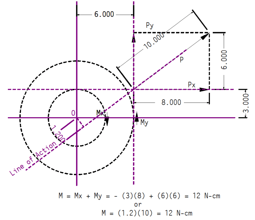
Vector analysis also obscures the fact that a moment is the product of the force and the perpendicular moment arm from the point of application to the line of action of the force. This is illustrated in An Example of 2D Moment Computation. In fact that’s the key problem to vector analysis: the student gets bogged down in setting up the problem rather than understanding its nature.
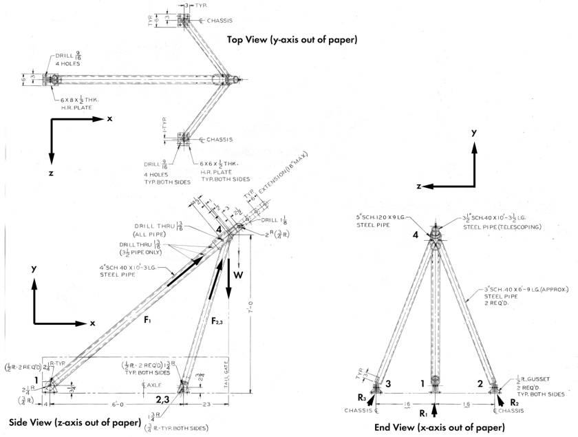
Problems–especially three-dimensional ones–are best left to numerical methods and emphasis on two-dimensional problems for basic understanding would be a better approach. The last example I’d like to give is An Example of 3D Vector Statics With a Simple Truss. Here we have a problem where (as you can see in the example itself) the vector solution is just too much for the problem; we could either a) use a numerical method or b) split the problem into two two-dimensional problems, one in the x-y plane and the other in the 2-3-4 plane.
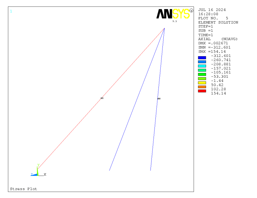
The solution in ANSYS (I know this is an old version, we run on a low budget on this site) is below.
I’m aware that vector analysis is well embedded in the teaching of mechanics, but I think it’s time to take a serious look at the problem.
Bring Back Graphical Methods
One hallmark of engineering practice in the past was the use of graphical methods to resolve forces and perform other tasks which would be computationally expensive. The advent of the calculator and later the computer into the profession gave the impression that graphical methods were a thing of the past.
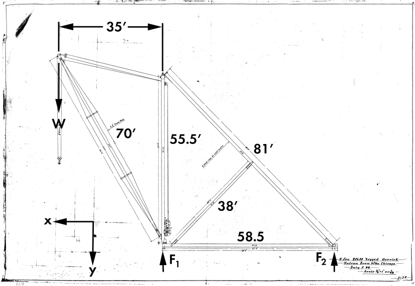
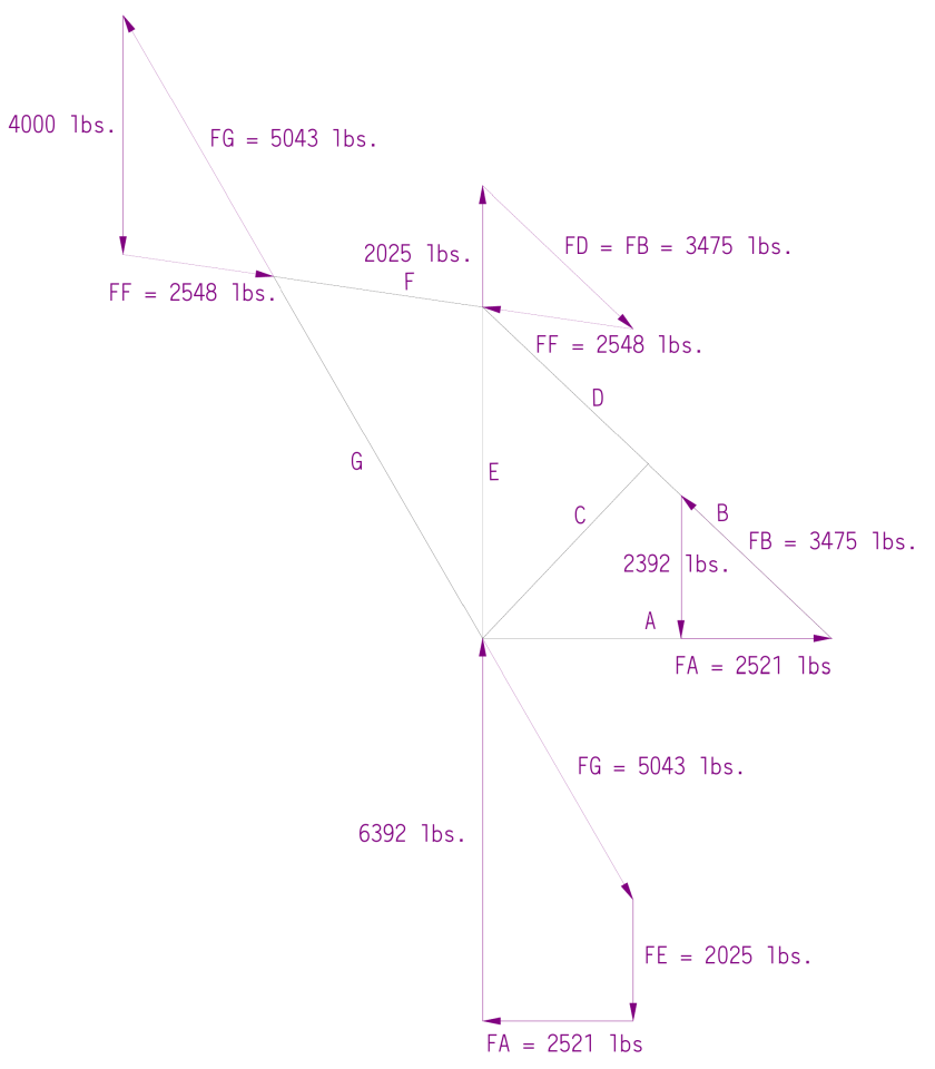
With CAD that’s not the case: we can solve problems with the same precision in CAD we do with either vector analysis or “old coot” statics. An example of this comes from the very first example shown; the graphical solution is given in the article Stiff Leg Derrick Part II: Truss Analysis, and can be seen below. The magnitudes were measured in CAD and the directions were done using the basic derrick layout in CAD.
Graphical methods will assist visualisation and give students a better feel for the problem, both of which they need in their development as engineers.
Distributed Loads and Concentrated Resultants
This comes out of my geotech teaching but also Fluid Mechanics as well: my students struggled with the transition from distributed loads to concentrated resultants. And the distributions were the usual ones we see in geotech and Fluid Mechanics: linear, either uniform, triangular, or trapezoidal. I’m not sure what the solution is but there are two things we need to consider: a) the aforementioned vector statics and b) the inclusion of algebraically complex loadings with polynomial or other higher order equations. As a practical matter it’s unlikely that a complex loading encountered in practice will obey these equations but will more likely require a stepped type of loading of some kind, which in turn begs a numerical solution.
Keep Basic Fluid Mechanics Basic
Fluid Mechanics has experienced much of the same transition as solid mechanics. From books like Hydraulics and Fluid Mechanics to those we usually teach from now, an emphasis on practical fluid mechanics has been lost. In my own career I have found that many of the problems I had would have been much easier to see if the curriculum I was taught under had stuck with a more basic approach (and books which emphasise that do exist, as you can see from my own course.) What we need is to do the following: a) save much of the more theoretical treatment for an advanced course, paralleling that of mechanics of materials, and b) integrating that type of material into basic Computational Fluid Dynamics, which is a necessity for many fluid mechanics problems.
One other thing worth mentioning is that, in the past, solid and fluid mechanics were more integrated, as you can see in books from Smith’s Mechanic to Mechanics by S.P. Strelkov. We might consider some of this if we decide to seriously rearrange how we teach these subjects.
Putting a Wrap
This is not meant to be an all-inclusive list, and I realise that some of these suggestions will be controversial. Today it’s fashionable in higher education, as it has been down the line for many years, to emphasise the pedagogy methods as opposed to the content. But a simpler, more straightforward approach to subject would lend itself to easier pedagogy; the two aren’t unrelated. The tendency to push practitioners out out teaching–one driven in part by our accreditation process–has left many with an unclear understanding of what is required of engineers once they graduate. There are many issues we face; this piece is only meant to start the conversation, not finish it.
One of the reasons I was interested in teaching Statics at Lee University was because I was continually disappointed at my students’ memory of their statics. Statics is crucial in the design and analysis of geotechnical structures, and most of the problems–at the undergraduate level at least–aren’t that involved, or at least I thought they weren’t. A great deal of the problem is that geotechnical statics usually involves converting distributed loads into resultants, which Statics–and Mechanics of Materials for that matter–generally associate this with beam problems, not always the case with geotechnical problems.
Another culprit is that Statics, in the U.S. at least, is a vector proposition from the start. At the University of Tennessee at Chattanooga where I taught, it was called “Vector Statics,” which gives the game away early. (At Lee we use the same book and teach the same material, but simply title it “Statics.”)
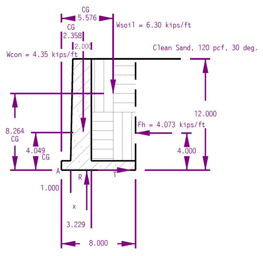
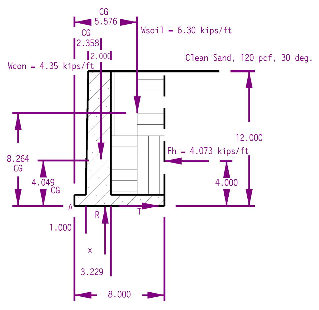
But what if we applied a vector approach to a simple geotechnical problem? That’s what we’re going to do here with a concrete gravity wall. I will use the method outlined in my post A Simplified Method to Design Cantilever Gravity Walls. You can refer to the theory there, I will try to keep it to a minimum. The wall is pictured at the top of the post, I will reproduce it below.
Analysing Overturning
We have three forces acting on the wall:
The weight of the gravity wall itself, Wconc
The weight of the soil trapped by the heel of the wall, Wsoil
The lateral force of the soil on the wall, Fh
Forces 1 and 2 are determined by computing the cross-sectional area of the concrete and soil and multiplying each by the unit weight as shown above, and then converting the result to a vector force and placing it at the centroid of the area (another Statics topic.) Instead of the “manual” approach in A Simplified Method to Design Cantilever Gravity Walls, the was was drawn in CAD and both the areas and centroids were determined automatically. You can see the magnitudes and locations of those resultants above.
The lateral force of the soil is computed using Rankine’s theory. The first thing is to determine the working internal friction angle of the soil by applying the Shear Mobilisation Factor SMF. Assuming an SMF of 2/3, that friction angle changes from the 30 degree one shown above to a 21.05 degree one, which is applied to the formula for Rankine active pressures for level backfill,
(1)
Doing that results in a kh = .471. The force on the wall is then determined by the formula
(2)
The division by two reflects the fact that soil effective stress (and thus lateral earth pressure) increases linearly with depth (like a fluid,) creating a triangular distribution (yet another concept from Statics.)
At this point there the resisting forces R and T are not defined. The forces themselves are easily computed by summing forces in the x and y directions. Doing this, we have
(3a) (3b)
The location of F–along the surface of the footing–is evident. The location of R is not; it is some distance x from the toe (Point “A”) of the footing. We can obtain x by summing moments around Point “A,” and with a vector method that means taking cross products of the moment arms with the forces.
Converting both the moment arms r and the forces to vector notation yields the following:
Concrete Weight: r = 2.358 i + 4.049 j, Wcon = −4.35 j
Soil Weight: r = 5.576 i + 8.264 j, Wsoil = −6.30 j
Lateral Earth Pressure: r = 8 i + 4 j, Fh = −4.073261616 i
Vertical Footing Force: r = x i, R = 10.65 j (Equation (3a))
The force T does not enter into this because its line of action runs through Point “A,” thus its moment is zero as its moment arm is zero.
The cross product moments around the toe (Point “A” in the drawing) are as follows:
Concrete Weight:
Soil Weight:
Lateral Earth Pressure:
Vertical Footing Force:
Summing these moments,
(4)
Solving yields x = 2.732′. At this point we need to determine whether this is an acceptable location or not for the force. The goal is for the pressure to be positive (downward) along the entire surface of the footing. There are two ways of determining this:
We will do the latter. The middle third of this foundation falls between 2.67′ < x < 5.33′, so the vertical footing force is within the middle third (barely.) As I noted in A Simplified Method to Design Cantilever Gravity Walls, “In this case we make a common assumption that, as long as the resultant force of the wall is within the kern and there are no negative pressures on the base, overturning will not be experienced. It is certainly possible to do an explicit overturning analysis to check this result.”
Analysing Sliding
With the lack of keys or deep foundations, the only lateral resistance to sliding is the friction force T. We computed that force based on Equation (3b,) but in reality that force cannot exceed–and there should be a factor of safety in that inequality–the frictional force possible, which is defined by the equation
(5)
in which case
(6)
Equation (5) is written in “mechanical engineers format.” Geotechnical engineers understand all too well the concept of a friction angle. In my post Explaining the Relationship Between the Coefficient and the Angle of Friction I relate the two from a non-geotech standpoint; we can turn Equation (5) into a more “geotech-friendly” form by noting that
(7)
Let us assume that the value of is the same under the wall as next to the wall, and let us also assume that the friction angle between the base and the soil is the same as the friction angle of the soil overall, as was done in A Simplified Method to Design Cantilever Gravity Walls. That being the case, . Substituting into Equation (5,) . The factor of safety from Equation (6) is thus , which is barely over the minimum criterion for usual loads given in A Simplified Method to Design Cantilever Gravity Walls.
Observations
The use of vectors for this problem is overkill from a computational standpoint. It also requires locating the centroid/CG of the two regions in both the x- and y-directions, although with using CAD this is trivial. On the other hand doing it using vectors is more “bullet proof” in that the student is not required to “think” but just “plug and chug” without having to identify lines of action and perpendicular moment arms.
The fact that the word “barely” appears in both analyses should inspire some additional conservatism in the design. The simplest way to improve the situation would be to move the heel to the right, which would shift the resisting forces away from the toe (and thus increase their resisting moment) and also put the footing force resultant deeper into the middle third.
Both bearing capacity and settlement of the wall’s foundation, the methodology for which are discussed in A Simplified Method to Design Cantilever Gravity Walls, are beyond the scope of this post. Also beyond the scope of this post is the structural design of the wall and of course the global stability of the wall as well.
My post Getting to the Legacy of B.K. Hough and his Settlement Method got a good amount of interest. Unfortunately it left several “loose ends,” some of which is because we don’t have full information on some of Hough’s methodology, and others because we don’t have full information on the FHWA’s thinking in their resurrection of the method. The objective of this post is to clear up some of these loose ends, especially the latter.
What we needed was some additional information on the background for both Hough’s work and the FHWA’s interpretation of that work. That information came from an unexpected source: the FHWA’s Design and Construction of Driven Pile Foundations, 2016 Edition. This has been available on vulcanhammer.info just about since it was first published. Now some of you are asking, “Why is this guy waiting until now to come out with stuff he’s had for years? Doesn’t he read the material he offers for download?” In my defence, I didn’t expect the solution to come from the driven pile manual, since it’s primarily a shallow foundation issue. It’s there because it’s proposed for use with groups of driven piles in cohesionless soils.
With all that said let’s look at some of the issues this “new” source tackles.
The SPT Correction Issue
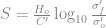
The basic equation for Hough’s method is similar to that used for one-dimensional consolidation settlement and is
(1)
where
settlement of cohesionless soil layer
layer thickness
compression coefficient
effective stress at the centre of the layer
effective stress at the centre of the layer plus the induced stress from the surface at the centre of the layer
Hough’s Method may or may not have used a 60% (N60) efficient hammer to develop the method. It’s entirely possible but Hough (1959) doesn’t say what type of hammer he used to develop the method.
The FHWA implementation of Hough’s method included an SPT correction for overburden, which was absent in Hough (1959.)
An absence of any mention of Hough (1969,) where he modified the values.
The lack of an attempt to convert the chart to equations. My original post demonstrates how this can be done, using the method of Hough (1969.)
Cheney and Chassie (2002) report that FHWA experience with this method indicates the method is usually conservative and can overestimate settlements by a factor of 2. This conservatism is attributed to the use of the original bearing capacity index chart from Hough (1959) which was based upon SPT donut hammer data. Based upon average energy variations between SPT donut, safety, and automatic hammers reported in technical literature, Figure 7-43 now includes a correlation between SPT N values from safety and automatic hammers and bearing capacity index. The safety hammer values are considered N60 values. This modification should improve the accuracy of settlement estimates with this method.
The following should be noted about these changes:
The assumption that Hough used a “donut” hammer is a reasonable one based on the technology of the time, but it’s still an assumption. Hough doesn’t tell us the kind of SPT hammer he used, or even how he came up with the C’ values shown above.
The chart above (Figure 7-43) shows the correlation for three types of hammers: donut, safety, and automatic hammers (which now “rule the roost” in testing.) However, it still insist that the safety hammer values should be corrected for overburden, something else absent from Hough’s study.
There is still no awareness of Hough (1969.)
So we can say that we have, perhaps, made some progress toward a solution, but at this point we are not quite where we would like to be.
My Thinking on the Way Forward
We usually think in terms of progress in this field in terms of peer-reviewed articles. But we’ve had the peer-reviewed articles, the experts weigh in on what they mean, and another set of experts try to make things better. My own solution to this problem would run like this:
Let’s accept the FHWA’s idea that Hough used a donut hammer for his original work. Donut hammers have a “standard” efficiency of 45%. To get the SPT blow counts to an N60 value (60% efficiency) we need to divide the donut SPT values by 60/45 = 4/3. (That’s what’s going on in the graph above.)
Let’s use Hough’s method as he presented it in Hough (1969) and assume that those values too came from donut hammers.
Let’s lose the overburden correction; it wasn’t in the original and I don’t see how one can justify putting it into this method.
If we implement all of this, the chart now looks like this:
If formulae are preferred (and that’s normally the case these days) they will again be in the form
(2)
and the coefficients will be as follows:
Soil Type
A
B
Organic Silt, Little Clay
7.22
0.0305
Inorganic Sandy Silt
18.27
0.0279
Very Well Graded Fine to Coarse Sand
22.86
0.0270
Well Graded Clean Fine to Coarse Sand
28.22
0.0289
Well Graded Silty Sand and Gravel
32.85
0.0289
Uniform Clean Inorganic Silt
37.02
0.0294
Very Uniform Clean Medium Sand (Similar to Std. Ottawa)
58.66
0.0299
The “B” coefficients run in a fairly narrow range and have an average of 0.0289. It’s possible using this or a more sophisticated method to apply the same value of B to all of the soils.
Any comments from those of you who have used Hough’s Method, or have research on the topic, would be greatly appreciated.
References
Hough, B.K. (1959). “Compressibilty as the Basis for Soil Bearing Value,” Journal of the Soil Mechanics and Foundations Division, ASCE, Vol. 85, Part 2.
Hough, B.K. (1969). Basic Soils Engineering. Second Edition. New York: Ronald Press Company.


 (1)
(1) (2)
(2) (3a)
(3a) (3b)
(3b)![\left [\begin {array}{ccc} i&j&k\\{\medskip} 2.358& 4.049&0 \\{\medskip}0&- 4.35&0\end {array}\right ] = -10.257 k](https://s0.wp.com/latex.php?latex=%5Cleft+%5B%5Cbegin+%7Barray%7D%7Bccc%7D+i%26j%26k%5C%5C%7B%5Cmedskip%7D+2.358%26+4.049%260+%5C%5C%7B%5Cmedskip%7D0%26-+4.35%260%5Cend+%7Barray%7D%5Cright+%5D++%3D+-10.257+k+&bg=ffffff&fg=777777&s=0&c=20201002)
![\left [\begin {array}{ccc} i&j&k\\{\medskip} 5.576& 8.264&0\\{\medskip}0&- 6.3&0\end {array}\right ] = -35.129k](https://s0.wp.com/latex.php?latex=%5Cleft+%5B%5Cbegin+%7Barray%7D%7Bccc%7D+i%26j%26k%5C%5C%7B%5Cmedskip%7D+5.576%26+8.264%260%5C%5C%7B%5Cmedskip%7D0%26-+6.3%260%5Cend+%7Barray%7D%5Cright+%5D+%3D+-35.129k+&bg=ffffff&fg=777777&s=0&c=20201002)
![\left [\begin {array}{ccc} i&j&k\\{\medskip}8&4&0\\{\medskip}- 4.073&0&0\end {array}\right ] = 16.293k](https://s0.wp.com/latex.php?latex=%5Cleft+%5B%5Cbegin+%7Barray%7D%7Bccc%7D+i%26j%26k%5C%5C%7B%5Cmedskip%7D8%264%260%5C%5C%7B%5Cmedskip%7D-+4.073%260%260%5Cend+%7Barray%7D%5Cright+%5D+%3D+16.293k&bg=ffffff&fg=777777&s=0&c=20201002)
![\left [\begin {array}{ccc} i&j&k\\{\medskip}x&0&0\\{\medskip}0& 10.65&0\end {array}\right ] = 10.65 x k](https://s0.wp.com/latex.php?latex=%5Cleft+%5B%5Cbegin+%7Barray%7D%7Bccc%7D+i%26j%26k%5C%5C%7B%5Cmedskip%7Dx%260%260%5C%5C%7B%5Cmedskip%7D0%26+10.65%260%5Cend+%7Barray%7D%5Cright+%5D+%3D+10.65+x+k+&bg=ffffff&fg=777777&s=0&c=20201002)
 (4)
(4) (5)
(5) (6)
(6) (7)
(7) is the same under the wall as next to the wall, and let us also assume that the friction angle between the base and the soil is the same as the friction angle of the soil overall, as was done in
  . Substituting into Equation (5,)
  . The factor of safety from Equation (6) is thus
  , which is barely over the minimum criterion for usual loads given in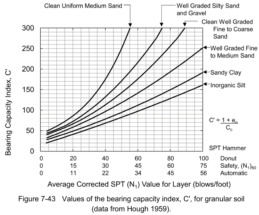
 (1)
(1) settlement of cohesionless soil layer
 layer thickness
 compression coefficient
 effective stress at the centre of the layer
 effective stress at the centre of the layer plus the induced stress from the surface at the centre of the layer
 . My criticisms of the FHWA’s implementation of the method in the post
  values.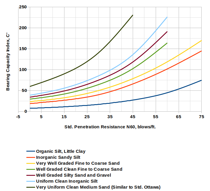
 (2)
(2) vulcanhammer.net