There are some things in geotechnical engineering that don’t get really good (if any) coverage in many textbooks, which means that those who go on into that part of civil engineering are blindsided by their appearance. One of these is the “line of optimums” approach for compaction evaluation. The only formal textbook I know of that covers it is Soils in Construction, for which I must credit my co-author, Lee Schroeder. It also appears in the Soils and Foundations Reference Manual.
The line of optimums approach seeks to answer a key question in compaction: how much compactive energy is necessary to effect a given compaction? We have the Standard Proctor and the Modified Proctor test, but when we’re trying to determine a specific compactive effort for a particular soil and project, we need more flexibility.
I discuss this in my class video for Soil Mechanics: Compaction and Soil Improvement, but let’s consider an example, in this case from Rebrik (1966).
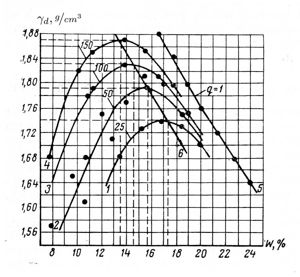
The lines on the chart are as follows:
- Lines 1, 2, 3 and 4 represent compaction curves for a soil, but with a different number of blows (25, 50, 100 and 150, as shown in the chart.) As is customary, the plot is the water content (x-axis) against the dry density (y-axis,) although in American practice this is usually the dry unit weight.
- Line 5 is the “zero air voids curve,” i.e., the curve where the degree of saturation S = 100%.
- Line 6 is a “trendline” of the peak compaction dry densities, a “line of optimums.”
At this point, we will show a more “contemporary” approach to the line of optimums method than what’s in the book, which dates back to the semilog paper era. The first thing we do is to switch the x-axis from the water content to the number of blows for each compaction. We then plot this against the y-axis of the maximum dry density for each compaction, the result is tabulated as follows:
| Compactive Blows | Dry Density, g/cm3 |
| 25.00 | 1.7407 |
| 50.00 | 1.7936 |
| 100.00 | 1.831 |
| 150.00 | 1.8699 |
Now we can plot this in a spreadsheet and estimate a trendline for the best fit. The result is plotted as follows:
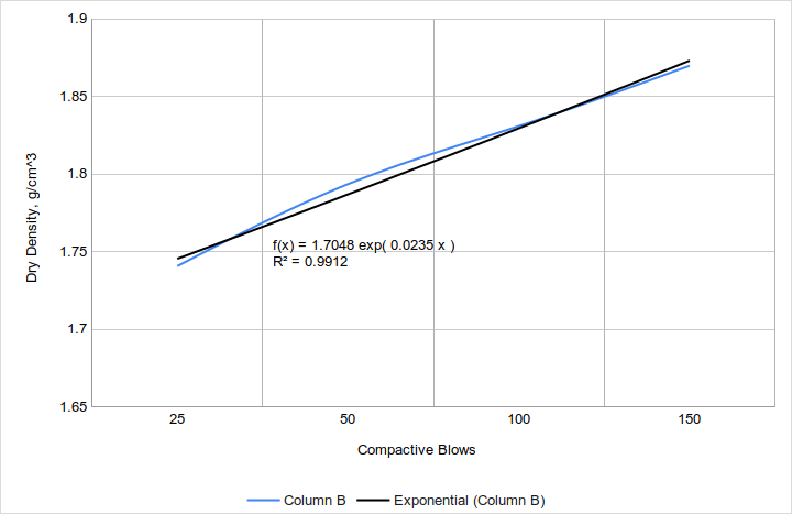
As it happens the power correlation turns out to have the highest R2 value. The book’s graph implies an exponential fit, but the variance in R2 between them is not great. Using the spreadsheet’s trendline feature gives the designer more flexibility in reducing the data. An explanation of that trendline feature–and curve fitting in general–can be found at Least Squares and Curve Fitting.
At this point we have a problem: we do not have the compactive effort for the differing blow counts. This is easily remedied because Equation 8.5 in Soils in Construction shows that, if the compaction mould, volume of soil, number of lifts and impact energy are all the same (a reasonable assumption in this case,) then the number of compactive blows is directly proportional to the compactive energy.
With that information in hand, we can take an actual compaction method and lift depth and estimate the maximum dry density we can expect. If it is not adequate for the task, we can either use a different compaction method or revise our design for a lower compactive dry density. We also need to determine a reasonable relative compaction, which will reduce this value to one which we can expect to happen during actual compaction.
The line of optimums method is a good one for compaction evaluation, and we hope that this little presentation helps you to understand it.
Reference
- Rebrik, B.M (1966) Vibrotekhnika v burenii (Vibro-technology for Drilling.) Moscow, Russia: Nedra.