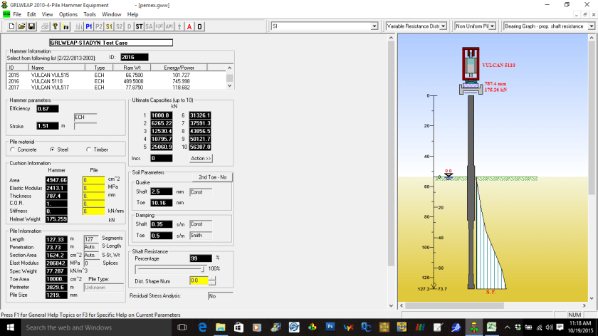
While looking through some files, I found these from the original STADYN project, from the comparison case with GRLWEAP. I’m passing these along to give you an idea of the graphical output of this program. My thanks to Jonathan Tremmier of Pile Hammer Equipment for allowing me to use this copy of GRLWEAP.
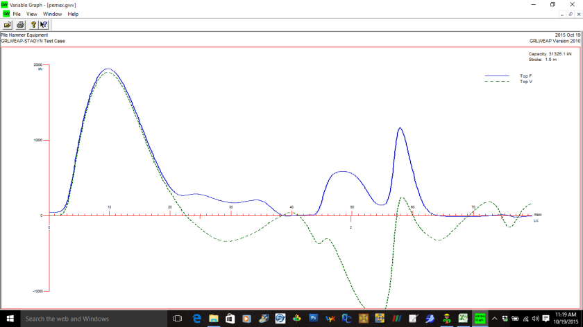
This is the “main screen” of GRLWEAP, giving a schematic view of the hammer/pile/soil system and allowing for input of parameters.This is the “bearing graph” output of the program, also giving a graphical representation of the system.This is the force-time and impedance*velocity-time trace for the pile head. Comparing the two is an important element when this data is gathered in the field.
It’s been a while since the last post on this subject; this has slowed things down. But in the course of getting started again a little “side trip” shows a good illustration of how sometimes determining the engineering properties of a structural element–in this case a driven concrete pile–can be challenging.
The test case for this is the FHWA’s A Laboratory and Field Study of Composite Piles for Bridge Substructures. All of the information in this piece comes from that report. The report dates back to 2006 and the actual field work earlier in the decade. One of the test cases involves a bridge replacement in Hampton, VA, as shown above.
The study involved the installation and testing of three different types of piles, as shown below. We’ll concentrate on the prestressed concrete pile on the left.
Pile cross-sections tested at the Route 351 Project
The prestressed concrete pile was a 610 mm square solid pile. This means that the cross-sectional area is . The pile was 18 m long, as shown below.
Elevation view and instrumentation plan for concrete pile.
Stress-strain curves were developed for the three materials, and these are shown below.
Stress-strain curves for the pile materials.
From the stress-strain curve for the concrete alone (and we usually assume that the concrete governs the pile elastic properties for compression at least) the curve would indicate that the modulus of elasticity is somewhere around . The diagram below, however, indicates that those involved in the project determined the modulus of elasticity to be around .
Axial load-axial strain behavior of test piles.
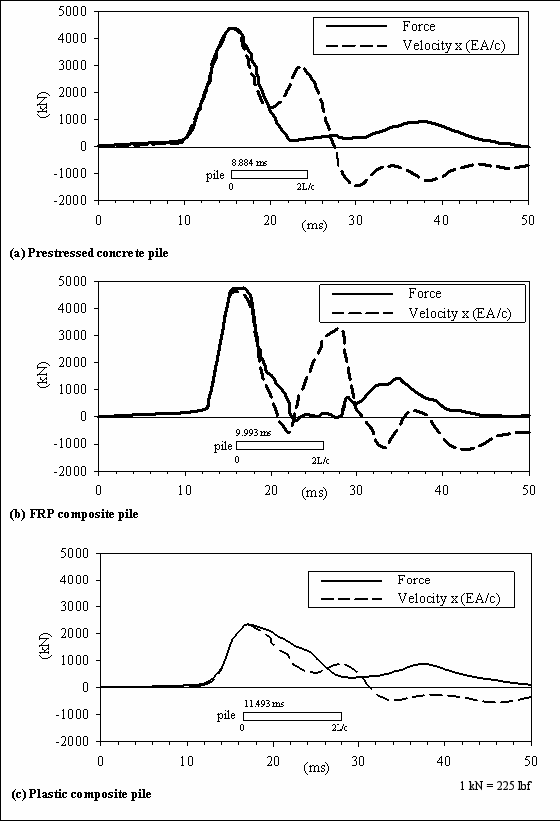
The interest from the STADYN standpoint is to obtain a force-time and velocity-time curve from the Pile Driving Analyzer, and this is certainly forthcoming:
PDA Results for Test Piles
The value of was probably determined from the two force peaks. The first force peak is the impact of the hammer on the pile and the second is the reflection of that impact from the toe. Both are compressive and the second is strong, which indicates a high level of toe resistance.
As is typical with PDA output, the force and the velocity (multiplied by the impedance) are plotted together. Unfortunately the document does not give the impedance for this case, so it’s necessary to back compute the impedance. Since we have a reasonably good idea of from the PDA, and the impedance Z is
we can determine the impedance. Solving for c from ,
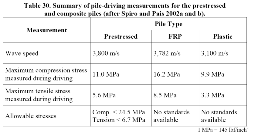
We need to pause at this point and note that other values of acoustic speed are implied in the data. For example, the following table states an acoustic or wave speed of 3800 m/sec.
Acoustic speeds and other results of pile driving and dynamic testing.
Before and after the test, PIT (Pile Integrity Tests) were run on the pile. The results are below.
Results of PIT tests.
Converted to SI units, the acoustic or wave speed becomes 4037 m/sec, which is fairly close to the PDA tests. The PDA results will be used for the remainder of this piece.
In any case, using the EA values from the earliest part of the test, the impedance is
The data was extracted from the PDA results. The force values could be used “as is.” The velocities were in reality the product of the velocity and the impedance, so the dashed line values were divided by the impedance just obtained to yield a velocity. Unfortunately, when this was put into STADYN, the velocities that resulted–even in the early stages of impact, where semi-infinite pile conditions predominate–the velocities of the program varied from the velocities extracted from the data by a factor of two. Checks in the program did not show any change in the way the program executed the algorithm from earlier runs, but the impedance values the program was yielding were considerably different from the one above.
In an attempt to sort things out, it is good to start by noting that the acoustic speed is computed by the equation
The report states that the pile was poured to normal Virginia DOT specifications. A fair assumption is that the density or unit weight of the concrete is close to normal, or . That being the case, the computed acoustic speed from the values of Young’s modulus E (which is necessary to put into Pa for unit consistency) and the density assumed yields
Something is clearly wrong here, and the most probable culprit is the modulus of elasticity of the concrete. A common way to estimate the modulus of elasticity of concrete in MPa is to use the formula
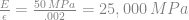
where is the 28-day compressive strength of the concrete. The report gives this to us at the time of the load tests as 55 MPa, which yields a modulus of elasticity of
This is considerably higher than the earlier data would indicate. It’s worth noting the the specifications for the pile set a minimum value for as 35 MPa; this indicates that the values of Young’s Modulus for concrete in piles can vary widely.
Another–and given the data probably a stronger–approach to compute the value of Young’s Modulus is to back compute it from the acoustic speed (which is known within reasonable values) and the density (see assumption above.) Solving the basic equation for acoustic speed for Young’s Modulus yields
Substituting our values yields
The impedance from this would be
Applying values along this line and recomputing the velocities, the results of the STADYN program and the actual PDA results were much closer.
Conclusions
The reason for the discrepancy in Young’s Modulus–and thus the pile impedance–is unclear. It may be due to rate effects on the elastic response to concrete, or it may be due to other factors.
Wave equation analysis are typically run according to “standard” material properties. Those who run these should be aware that, with concrete and wood, those properties may not reflect the properties of what actually gets driven into the ground.
Any force- and velocity-time data such as are produced by the PDA should have their axes labelled properly (with both force and velocity) or with the impedance reported.
Even with controlled research projects, discrepancies can arise in the data which can impede (pun somewhat intentional) the use of the data, and careful analysis is necessary to avoid problems such as was seen in this situation.
Abstract: The STADYN program was developed for the analysis of driven piles both during installation and in axial loading. Up until now the test cases used were in predominantly cohesive soils. In this paper, the expansion of the program’s use into predominantly cohesionless stratigraphies has required consideration of two important factors. The first is the difference between strain-softening in clays as opposed to sands, and additionally static vs. dynamic strain effects. This requires a review of the whole concept of the “magical radius” for pile elasticity. The second is the effect of dilatancy on the response of the pile to axial loading. Both of these are discussed in this paper, and test cases are presented to illustrate the application of the program to actual driven piles.
Abstract: Although it is widely understood that soils are non-linear materials, it is also common practice to treat them as elastic, elastic-plastic, or another combination of states that includes linear elasticity as part of their deformation. Assuming hyperbolic behavior, a common way of relating the two theories is the use of strain-softened hyperbolic shear moduli. Applying this concept, however, must be done with care, especially with geotechnical structures where large stress and strain gradients take place, as is the case with driven piles. In this paper a homogenized value for strain-softened shear moduli is investigated for both shaft and toe resistance in clays, and its performance in the STADYN static and dynamic analysis program documented. A preliminary value is proposed for this “average” value based upon the results of the program and other considerations.
In our last STADYN post we discussed the addition of factors to take into account adhesion phenomena with cohesive soils. In this post the addition of a more mundane but nevertheless important parameter for impact pile hammer systems is done: consideration of plastic losses in hammer and pile cushions, and interfaces as well.
Most impact pile hammers use some kind of hammer cushion; additionally, concrete piles are almost always driven with pile cushion at the pile head. Cushions of both kinds are subject to significant plastic deformation and generation of heat. There are several possibilities of modelling these elements in a simulation such as STADYN.
The first is to use velocity-dependent (viscous) damping to simulate the dissipation of energy. STADYN in its current form has no velocity-dependent parameters; to add these would involve some major changes in the code, and in any case the testing of cushion material does not produce a result that would indicate such a property.
The second is to use an elastic-purely plastic approach similar to the one used in the soils. The problem with this is that it would “flat-top” the impulse to the pile, and there is no evidence that the cushion material fails in this way.
The third is to use a “coefficient of restitution” approach, where the rebound of the cushion takes place at a different stiffness than the compression. This is illustrated in two variants below.
Cushion Models for Plastic Cushions (from Warrington (1988))
The conventional model dates back to Smith, and is still used in GRLWEAP. The ZWAVE model is described by Warrington (1988). In both cases the energy lost in the cushion is represented by the shaded area.
For STADYN the conventional model was adopted. Implementing this took a little more care in a finite element code than in finite-difference codes like WEAP and GRLWEAP but it was done. To accomplish this, it was necessary to compute the force in the cushion incrementally, as with plasticity the response is now path-dependent. When the cushion rebounded (i.e., the distance between the cushion faces increased from one step to the next) the rebounding stiffness is used. In this way multiple rebounds can be modelled properly.
Since the inverse methods do not model the hammer, the Mondello and Killingsworth case is not considered here. This leaves the other two cases, and these can be summarised very briefly.
The Finno (1989) case had a blow count increase from 15.8 to 17.0 blows/30 cm. For the SE Asia case, the blow count increased from 11.8 to 13.5 blows/30 cm. Additionally for the latter case comparisons with the pile head force and ram velocity vs. time tracks were produced.
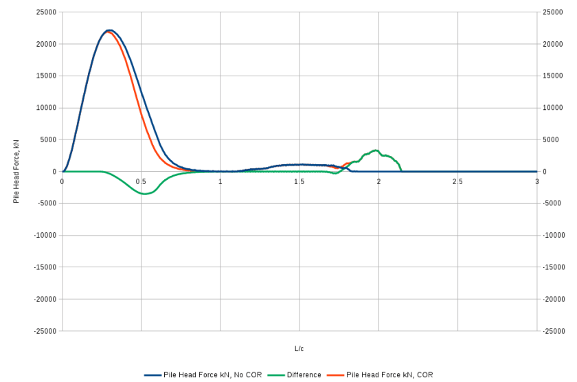
Pile Head Force
The pile head force until peak was identical, and then decreased more rapidly afterwards. There was an additional “kick” at 2L/c not present in the previous run.
Ram Point Velocity
The ram (point) velocity is the same until rebound, and then the ram is essentially stationary with the coefficient of restitution until 2L/c, after which the ram velocity in the two cases is very close. The sawtooth effect is mostly due to the “ringing” of the ram, i.e., a stress wave going up and down the ram.
While it is evident that the method of energy transfer is different with the addition of the coefficient of restitution, the actual effect of plasticity on the blow count is not great. This is probably due to two factors: most of the energy transfer takes place during compression of the hammer cushion, and both hammers are using micarta and aluminium, which has a relatively high coefficient of restitution (0.8). Nevertheless cushion losses are greater in materials such as plywood, which is used with concrete piles. It is to this type of pile that STADYN’s development now turns.


 . The pile was 18 m long, as shown below.
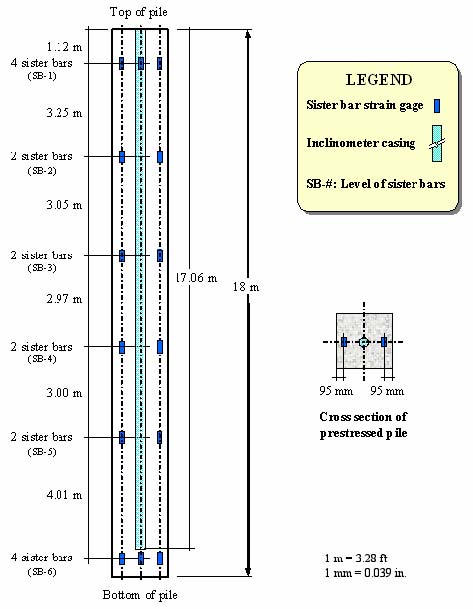
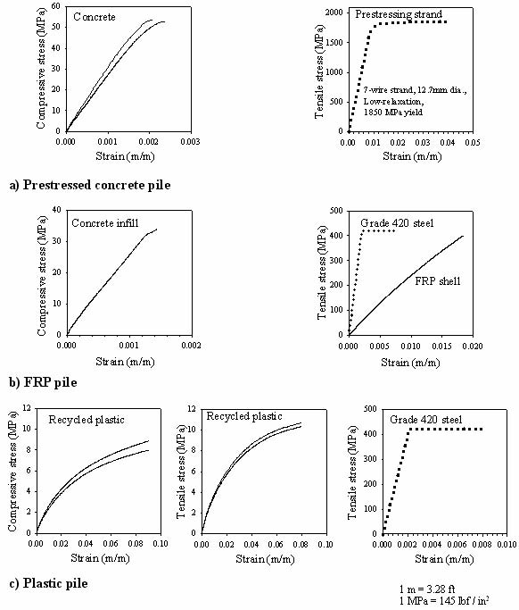
 . The diagram below, however, indicates that those involved in the project determined the modulus of elasticity to be around
  .
.
 was probably determined from the two force peaks. The first force peak is the impact of the hammer on the pile and the second is the reflection of that impact from the toe. Both are compressive and the second is strong, which indicates a high level of toe resistance.
 from the PDA, and the impedance Z is


 . That being the case, the computed acoustic speed from the values of Young’s modulus E (which is necessary to put into Pa for unit consistency) and the density assumed yields
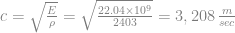

 is the 28-day compressive strength of the concrete. The report gives this to us at the time of the load tests as 55 MPa, which yields a modulus of elasticity of


 factors to take into account adhesion phenomena with cohesive soils. In this post the addition of a more mundane but nevertheless important parameter for impact pile hammer systems is done: consideration of plastic losses in hammer and pile cushions, and interfaces as well.

