TAMWAVE 5: Wave Equation Analysis, Overview and Initial Entry

With the static analysis complete, we turn to the wave equation analysis.  TAMWAVE (as with the previous version) was based indirectly on the TTI wave equation program.  Although the numerical method was not changed, many other aspects of the program were, and so we need to consider these.

Shaft and Toe Resistance

Most wave equation programs in commercial use still use the Smith model for shaft and toe resistance during impact.  Referencing specifically their use in inverse methods, Randolph (2003) makes the following comment:

Dynamic pile tests are arguably the most cost-effective of all pile-testing methods, although they rely on relatively sophisticated numerical modelling for back-analysis. Theoretical advances in modelling the dynamic pile-soil interaction have been available since the mid-1980s, but have been slow to be implemented by commercial codes, most of which still use the empirical parameters of the Smith (1960) model. In order to allow an appropriate level of confidence in the interpretation of dynamic pile tests, and estimation of the static response, it is high time that appropriate scientific models were used for pile-soil interaction, including explicit modelling of the soil plug for open-ended piles.

And that was in 2003…and the use of the Smith model in inverse methods was proceeded by its use in forward methods such as this one.  The model he is referring to from the mid-1980’s is, of course, the Randolph and Simons (1986) model, which was used in the ZWAVE program in the late 1980’s.  The details of this model were discussed in Warrington (1997).

The Randolph and Simons model is the one which is being used for the wave equation portion of this routine, as the static component was used for the ALP static axial pile analysis.  In converting the code from the Smith model to this one, there are some things that need to be understood.  We have discussed some of these earlier but others are as follows:

• Randolph and Simons (1985) used a visco-elastic-plastic model for both shaft and toe, the major difference being the location of the plastic slider for the shaft resistance (as is evident in the ZWAVE poster.)  Some contemporary “experimental” codes (such as Salgado, Loukidis, Abou-Jaoude and Zhang (2015)) add a series of springs and masses to replicate the soil mass that surrounds the piles.  While these doubtless enhance the performance of the models, we stuck with the simple visco-elastic-plastic model in TAMWAVE because these are better replicated in true 3D continuum models like STADYN.  1D code is good because of its simplicity, especially with an online routine like TAMWAVE.
• The 1′ segment/element lengths are carried over to the wave equation.  This is shorter than is customarily used even in commercial work but it saves interpolation of the properties along the shaft.
• The “Smith-type” damping constants are simply the damping of the element computed divided by its ultimate/plastic resistance.  Unlike the Smith model, however, the damping force does not vary with the instantaneous static resistance, but is simply the velocity multiplied by the damping constant and the ultimate resistance of that element, be it shaft or toe.  Thus different Smith type constants should be expected from the model being used.  Additionally, with the shaft resistance, the resistance of a shaft segment is limited to its ultimate static resistance.  This means that all additional damping forces must take place during elastic shearing of the soil surface.  Implicit in the Randolph and Simons model is that, once plasticity is achieved, the soil closest to the pile is effectively decoupled from the soil mass, and thus the pile movement can no longer radiate additional energy into the soil.  The result of this is that, as seen here, the Smith-type damping constants are much higher than one would normally assign.  Corte and Lepert (1985), in a direct comparison of the two models, note that the two give nearly the same result if the original Smith damping constants are multiplied by 7.5 for the new model.  Dividing the new result by this brings the damping constants much closer, especially in the lower reaches of the pile where most of the shaft resistance is found, although the ratio of 7.5 should be regarded as study-specific.  Bringing some rationality to the issue of damping constants would go a long way to improve the results of pile dynamics, forward and inverse, since variations of these have a significant impact on the results.
• We mentioned earlier that the toe quakes that resulted seemed high for this size of pile.  This may be due to the fact that “significant residual pressures are locked in at the pile base during installation (equilibriated by negative shear stresses along the pile shaft, as if the pile were loaded in tension.)  This will lead to a stiffer overall pile response in compression, and significantly higher end-bearing stresses mobilised at small displacements.”  (Randolph, 2003)  He goes on to state that “(f)or driven closed ended-piles the residual stress will be lower, but may still be as high as 75% of the base capacity…”  There are two ways to deal with this.  The first is to run the ALP program first and preload the base and shaft before using the resulting prestressed deflections to run the wave equation analysis.  This would be in effect a residual stress analysis (RSA,) which has been used in this field for many years.  The second is to use a “quick and dirty” method, i.e., to reduce the toe quake and thus simulate the higher toe stiffness and lower quake.  The latter was adopted in TAMWAVE, although one motivation from switching from P4XC3 to ALP was to make an RSA easier.  This is a possible point of future modification of the code.
• A change not related to the pile-soil interaction is the elimination of slack computation, as the pile is uniform and continuous (the hammer-cap and cap-pile interface is obviously inextensible.

Initial Wave Equation Input

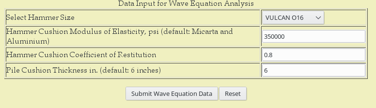
For our example the initial input of the wave equation is shown below.

Most of the data required has been carried over from the static analysis.  The hammer database was added in 2010; however, it was reordered in ascending rated striking energy order and a hammer was suggested using the “initial guess” criterion in the Soils and Foundations Handbook, which essentially suggests to set the initial hammer energy in ft-lbs at 8% of the ultimate capacity in pounds.  This is a “rule of thumb” designed to help students who, faced with a wave equation program for the first time, will have some idea of where to start, although there is no guarantee that the hammer will be either too large or small.  Since the energies are sorted, the user can move up or down the list to try another hammer.

The cushion material properties of the hammer, and the coefficient of restitution used to model cushion plasticity, are discussed (with sample properties) in the WEAP87 documentation.  No attempt was done to either convert coefficients of restitution to viscous damping or alter the rebound curve as was done in ZWAVE.  Pile cushion thickness is only input for concrete piles; the input is not shown for others.

References

In addition to those already cited, the following is included:

Corte, J.-F., and Lepert, P. (1986) “Lateral resistance during driving and dynamic pile testing.”  Proceedings of the Third International Conference on Numerical Methods in Offshore Piling, Nantes, France, 21-22 May.  Paris: Éditions Technip, pp. 19-34.