vulcanhammer.net

STADYN Wave Equation Program 12: A Case Study in the Modulus of Elasticity of Concrete Piles

Posted on 26 October 201926 May 2025 by Don Warrington

It’s been a while since the last post on this subject; this has slowed things down. But in the course of getting started again a little “side trip” shows a good illustration of how sometimes determining the engineering properties of a structural element–in this case a driven concrete pile–can be challenging.

The test case for this is the FHWA’s A Laboratory and Field Study of Composite Piles for Bridge Substructures. All of the information in this piece comes from that report. The report dates back to 2006 and the actual field work earlier in the decade. One of the test cases involves a bridge replacement in Hampton, VA, as shown above.

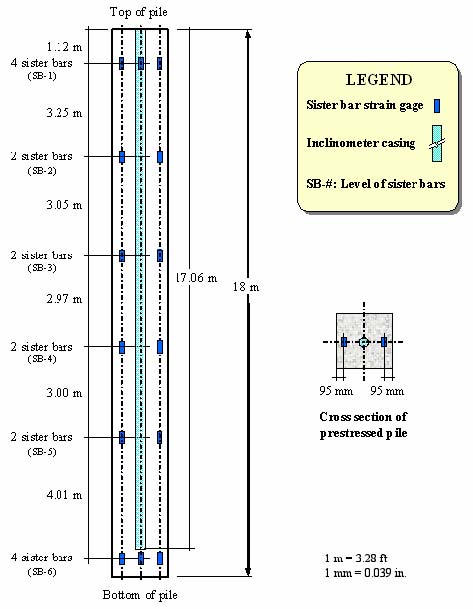
The study involved the installation and testing of three different types of piles, as shown below. We’ll concentrate on the prestressed concrete pile on the left.

Pile Profiles Figure 110.png — Pile cross-sections tested at the Route 351 Project

The prestressed concrete pile was a 610 mm square solid pile. This means that the cross-sectional area is $0.3721\,m^2$ . The pile was 18 m long, as shown below.

fhwa-hrt-04-043 — Elevation view and instrumentation plan for concrete pile.

Stress-strain curves were developed for the three materials, and these are shown below.

Stress-strain curves for the pile materials.

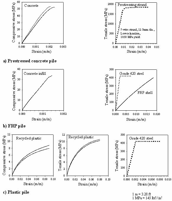
From the stress-strain curve for the concrete alone (and we usually assume that the concrete governs the pile elastic properties for compression at least) the curve would indicate that the modulus of elasticity is somewhere around $\frac{E}{\epsilon} = \frac {50\,MPa}{.002} = 25,000\,MPa$ . The diagram below, however, indicates that those involved in the project determined the modulus of elasticity to be around $\frac {EA}{A} = \frac {8.2 \times 10^3\,MN}{.3721\,m^2} = 22,037\,MPa$ .

Axial load-axial strain behavior of test piles.

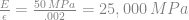
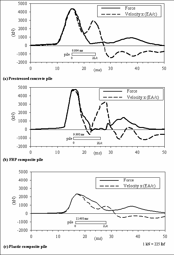
The interest from the STADYN standpoint is to obtain a force-time and velocity-time curve from the Pile Driving Analyzer, and this is certainly forthcoming:

PDA Results Figure 130.png — PDA Results for Test Piles

The value of $\frac{2L}{c} = 8.884\,ms$ was probably determined from the two force peaks. The first force peak is the impact of the hammer on the pile and the second is the reflection of that impact from the toe. Both are compressive and the second is strong, which indicates a high level of toe resistance.

As is typical with PDA output, the force and the velocity (multiplied by the impedance) are plotted together. Unfortunately the document does not give the impedance for this case, so it’s necessary to back compute the impedance. Since we have a reasonably good idea of $\frac {2L}{c}$ from the PDA, and the impedance Z is

$Z = \frac{EA}{c}$

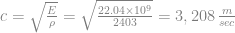
we can determine the impedance. Solving for c from $\frac {2L}{c}$ ,

$c = \frac{2 \times 18}{8.884\,ms} = 4052 \frac{m}{sec}$

We need to pause at this point and note that other values of acoustic speed are implied in the data. For example, the following table states an acoustic or wave speed of 3800 m/sec.

Table 30.png — Acoustic speeds and other results of pile driving and dynamic testing.

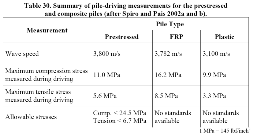
Before and after the test, PIT (Pile Integrity Tests) were run on the pile. The results are below.

Converted to SI units, the acoustic or wave speed becomes 4037 m/sec, which is fairly close to the PDA tests. The PDA results will be used for the remainder of this piece.

In any case, using the EA values from the earliest part of the test, the impedance is

$Z = \frac{EA}{c} = \frac {8.2 \times 10^6}{4052} = 2023 \frac{kN-sec}{m}$

The data was extracted from the PDA results. The force values could be used “as is.” The velocities were in reality the product of the velocity and the impedance, so the dashed line values were divided by the impedance just obtained to yield a velocity. Unfortunately, when this was put into STADYN, the velocities that resulted–even in the early stages of impact, where semi-infinite pile conditions predominate–the velocities of the program varied from the velocities extracted from the data by a factor of two. Checks in the program did not show any change in the way the program executed the algorithm from earlier runs, but the impedance values the program was yielding were considerably different from the one above.

In an attempt to sort things out, it is good to start by noting that the acoustic speed is computed by the equation

$c = \sqrt{\frac{E}{\rho}}$

The report states that the pile was poured to normal Virginia DOT specifications. A fair assumption is that the density or unit weight of the concrete is close to normal, or $\rho = 2403\,\frac{kg}{m^3}$ . That being the case, the computed acoustic speed from the values of Young’s modulus E (which is necessary to put into Pa for unit consistency) and the density assumed yields

$c = \sqrt{\frac{E}{\rho}} = \sqrt{\frac{22.04 \times 10^9}{2403}} = 3,208\,\frac{m}{sec}$

Something is clearly wrong here, and the most probable culprit is the modulus of elasticity of the concrete. A common way to estimate the modulus of elasticity of concrete in MPa is to use the formula

$E = 4700\sqrt{f'_c}$

where ${f'_c}$ is the 28-day compressive strength of the concrete. The report gives this to us at the time of the load tests as 55 MPa, which yields a modulus of elasticity of

$E = 4700\sqrt{55\,MPa} = 34,856\,MPa$

This is considerably higher than the earlier data would indicate. It’s worth noting the the specifications for the pile set a minimum value for ${f'_c}$ as 35 MPa; this indicates that the values of Young’s Modulus for concrete in piles can vary widely.

Another–and given the data probably a stronger–approach to compute the value of Young’s Modulus is to back compute it from the acoustic speed (which is known within reasonable values) and the density (see assumption above.) Solving the basic equation for acoustic speed for Young’s Modulus yields

$E = c^2 \rho$

Substituting our values yields

$E = 4052^2 \times 2403 = 39,454\,MPa$

The impedance from this would be

$Z = \frac{EA}{c} = \frac {39454\,MPa \times .3721\,m^2}{4052} = 3623 \frac{kN-sec}{m}$

Applying values along this line and recomputing the velocities, the results of the STADYN program and the actual PDA results were much closer.

Conclusions

The reason for the discrepancy in Young’s Modulus–and thus the pile impedance–is unclear. It may be due to rate effects on the elastic response to concrete, or it may be due to other factors.
Wave equation analysis are typically run according to “standard” material properties. Those who run these should be aware that, with concrete and wood, those properties may not reflect the properties of what actually gets driven into the ground.
Any force- and velocity-time data such as are produced by the PDA should have their axes labelled properly (with both force and velocity) or with the impedance reported.
Even with controlled research projects, discrepancies can arise in the data which can impede (pun somewhat intentional) the use of the data, and careful analysis is necessary to avoid problems such as was seen in this situation.

To commit to modeling software is a big decision for many firms, because it involves an investment of both money to purchase the program and time for employees to learn it. The decisions depends on the priorities of the office and its clients (or the clients they’d like to attract). In abbreviated form, the following […]

via Computer guidelines and Standards – MODELING PROGRAMS — Construction and architecture

Computer guidelines and Standards – MODELING PROGRAMS — Construction and architecture

Quote• Posted on 11 September 2019 by Don Warrington

Readers of this blog will know that my family goes back a long way visiting the Bahamas in general and the Abaco Islands in particular. We had some exciting times, almost sending our ship to the bottom and riding out a storm. This beautiful paradise, which looked like this when we visited: Now looks like […]

via Appeal for the Abaco Islands, and Mercy Chefs — Chet Aero Marine

Appeal for the Abaco Islands, and Mercy Chefs — Chet Aero Marine

Quote• Posted on 4 September 2019 by Don Warrington

Pile Driving Equipment

Pile Buck Ads 5: Vulcan 530 in Offshore Leaders

Posted on 13 August 201911 August 2019 by Don Warrington

For the last of the “Pile Buck Ads,” a photo of the Vulcan 530 hammer is featured in offshore stub-type leaders. The 530, introduced in 1978 for driving pipe piles offshore in the Gulf of Mexico, was and is used in a wide variety of pile driving projects. In this case it’s shown to be driving concrete cylinder piles, which have become common on larger bridge projects in the last quarter century.

Academic Issues

My Rimsky-Korsakov Moment in Academia

Posted on 1 August 201926 May 2025 by Don Warrington

In 1871, Nikolai Rimsky-Korsakov became a Professor of Practical Composition and Instrumentation at the St. Petersburg Conservatory. In retrospect, given the music he composed, this is not extraordinary. At the time, however, it was amazing. He was still in active service in the Russian Navy. More importantly, although he had had private music lessons and was very active with the “Five” (the group of Russian composers which gave Russian music its distinctive character,) he had never had any conservatory training! He worked hard to make up for this, and in doing so departed from the rest of the “Five” in making conservatory training part of being a Russian composer.

Russia is a very specific country; many strange things happen there and wherever Russians go. But maybe not as strange as we think: although I would never put myself in the rank of Rimsky-Korsakov in my own field, starting today I am a Lecturer in Mechanical Engineering at the University of Tennessee at Chattanooga. For those of you who have followed this site for a long time, this will seem quite odd, especially considering that one of the centrepieces of this site is the geotechnical courses that I have taught for nearly twenty years. My friend Jean-Louis Briaud, now President of the American Society of Civil Engineers, tried to encourage me with the fact that George Goble, who developed many of the tools we use in pile dynamics, started out as a mechanical engineer. But in reality some explanation is in order.

My entry into this field was through the equipment route, specifically the Vulcan Iron Works. That occasioned my first degree to be in Mechanical Engineering from Texas A&M University. Impact (and later vibratory) pile driving equipment is an unusual type of equipment to design and build. Basically it involves having a ram accelerate downwards due to gravity (with or without downward assist,) do this 30-120 times a minute, and stopped each time by deceleration which can be in the range of 150 g’s. This eliminates many common solution techniques used for mechanical design problems. Injected into an environment where service is frequently delayed and breakdown ruinous, it makes for many exciting moments in business.

The equipment, however, interacts with the pile which it is driving and the soil into which the pile is driven. Understanding this is really important in the proper design of the equipment. That realization came slowly but surely. By the time my family’s time at Vulcan was coming to an end, I was in graduate school, which ultimately resulted in a MS Degree in Civil Engineering. Before and during that time I presented several conference papers. But by the time I received my degree, my future in the deep foundations industry was uncertain.

Although I had other activities in the following years, that uncertainty was ended by three events. The first was starting this website; to make an educational resource like this you have to have some understanding of what you’re disseminating. The second was my involvement with Pile Buck and the compilation of two books: Sheet Pile Design by Pile Buck and Pile Driving by Pile Buck. The third was my teaching at the University of Tennessee at Chattanooga. When my MS thesis committee chairman retired, I taught Soil Mechanics and Foundations for one academic year (2001-2) thanks to another committee member, Dr. Edwin P. Foster, the Civil Engineering department head, who evidently thought enough of my abilities to bring me on.

The University had other ideas; due to some complex budgetary issues, they could not see their way clear to have me teach these courses as an adjunct for most of the last decade. It was not until 2009 that Ed Foster’s retirement and the concurrence of the current department head, Joseph Owino, meant that I was able to teach geotechnical courses at UTC on a consistent basis, something I have done ever since.

Dissertation Presentation_Page_01

Force Waves in Pile In 2011 I started my PhD in Computational Engineering, which is yet another engineering discipline. But both advanced degrees had one thing in common: they concerned pile dynamics, and that brings us to the marriage of mechanical and geotechnical engineering. It’s worth noting that E.A.L. Smith was Raymond’s Chief Mechanical Engineer, before George Goble came on the scene. Pile dynamics in any form involves things moving and moving fast, and civil engineers in general don’t find this very congenial. It’s an interdisciplinary field, one where mechanical engineers–and even equipment people–can make serious contributions.

Upon completing my PhD in 2016, my first new teaching assignment was the Fluid Mechanics Laboratory. This came as a shock to some, but things have worked out, and in any case an understanding of fluid mechanics is essential to geotechnical and mechanical engineer alike. But ultimately, as so many things are in academia, the full-time appointment (which many have pestered me about since I got my PhD) came from the Mechanical Engineering department due to internal considerations of the College of Engineering and Computer Science.

In going through all of this there’s one trend to be noted that also ties this into Rimsky-Korsakov’s story: the growth of the importance of formal education in the construction industry. In his case his conservatory experience didn’t endear him to some of his compositional colleagues, who were worried that European “formalism” would spoil the result. When I came into the family business in the late 1970’s many of our customers had little if any formal education beyond high school. Like some of the “Five” they accomplished great things. Today however the educational level of the construction industry–offshore and onshore alike–has risen, and has changed the nature of customer relations in a positive way.

Unlike many I’m not the first in my family to go to college. However, my people didn’t have a problem starting college: it was finishing it that was another story. When I completed my first degree is was the first completion in my family in sixty four years! The MS and PhD were without precedent, at least on my father’s side. While I am a strong believer that we build on what has gone before, we need to go beyond that, and an education is a way of achieving that result.

I am grateful for UTC’s confidence in me and in particular that of the department head (and my PhD advisor) James C. Newman, III. My teaching geotechnical courses will continue, as will my contributions to this site. Stay tuned.